
Introduction
In this post, we are going to look at some publicly available data to dig deeper into exploratory data analysis and machine learning techniques. I am going to start by fetching some data from the inter webs, this data is available at the FuelEconomy.gov site. This file has fuel economy data for all cars sold in the United States for several years.
Let’s start by loading the libraries we need:
suppressPackageStartupMessages({
  library(tidyverse)
  library(ggplot2)
  library(ggridges)
  library(ggthemes)
  library(ggrepel)
  library(data.table)
  library(here)
  library(skimr)
  library(scales)
  library(gridExtra)
  library(RColorBrewer)
})

here()
## [1] "/Users/nahuja/dev/r/site"
We’ll try to load the file directly from the site. This allows us to get the most recent data from the internet.
#temp <- tempfile()
#download.file("http://www.fueleconomy.gov/feg/epadata/vehicles.csv.zip", temp)
#unz(temp, "~/Downloads/vehicles.csv")
dt <- data.table::fread("~/Downloads/vehicles.csv", fill = TRUE)
#unlink(temp)

vehicles <- as_tibble(dt)
We have 46564 rows - that’s a lot of make and models.
Let’s take a look at what this data looks like using the excellent Skimr library for a succinct look.
skim(vehicles)
Table: Table 1: Data summary
| Name | vehicles |
| Number of rows | 46564 |
| Number of columns | 84 |
| _______________________ | |
| Column type frequency: | |
| character | 24 |
| logical | 1 |
| numeric | 59 |
| ________________________ | |
| Group variables | None |
Variable type: character
| skim_variable | n_missing | complete_rate | min | max | empty | n_unique | whitespace |
|---|---|---|---|---|---|---|---|
| drive | 0 | 1 | 0 | 26 | 1186 | 8 | 0 |
| eng_dscr | 0 | 1 | 0 | 46 | 17204 | 600 | 0 |
| fuelType | 0 | 1 | 3 | 27 | 0 | 14 | 0 |
| fuelType1 | 0 | 1 | 6 | 17 | 0 | 6 | 0 |
| make | 0 | 1 | 3 | 34 | 0 | 143 | 0 |
| model | 0 | 1 | 1 | 47 | 0 | 4872 | 0 |
| mpgData | 0 | 1 | 1 | 1 | 0 | 2 | 0 |
| trany | 0 | 1 | 0 | 32 | 11 | 41 | 0 |
| VClass | 0 | 1 | 4 | 34 | 0 | 34 | 0 |
| baseModel | 0 | 1 | 1 | 39 | 0 | 1431 | 0 |
| guzzler | 0 | 1 | 0 | 1 | 43838 | 4 | 0 |
| trans_dscr | 0 | 1 | 0 | 15 | 31520 | 53 | 0 |
| tCharger | 0 | 1 | 0 | 1 | 36708 | 2 | 0 |
| sCharger | 0 | 1 | 0 | 1 | 45568 | 2 | 0 |
| atvType | 0 | 1 | 0 | 14 | 41674 | 9 | 0 |
| fuelType2 | 0 | 1 | 0 | 11 | 44716 | 5 | 0 |
| rangeA | 0 | 1 | 0 | 11 | 44721 | 240 | 0 |
| evMotor | 0 | 1 | 0 | 51 | 44542 | 327 | 0 |
| mfrCode | 0 | 1 | 0 | 3 | 30808 | 56 | 0 |
| c240Dscr | 0 | 1 | 0 | 16 | 46423 | 6 | 0 |
| c240bDscr | 0 | 1 | 0 | 44 | 46429 | 8 | 0 |
| createdOn | 0 | 1 | 28 | 28 | 0 | 444 | 0 |
| modifiedOn | 0 | 1 | 28 | 28 | 0 | 284 | 0 |
| startStop | 0 | 1 | 0 | 1 | 31689 | 3 | 0 |
Variable type: logical
| skim_variable | n_missing | complete_rate | mean | count |
|---|---|---|---|---|
| phevBlended | 0 | 1 | 0.01 | FAL: 46323, TRU: 241 |
Variable type: numeric
| skim_variable | n_missing | complete_rate | mean | sd | p0 | p25 | p50 | p75 | p100 | hist |
|---|---|---|---|---|---|---|---|---|---|---|
| barrels08 | 0 | 1.00 | 15.27 | 4.39 | 0.05 | 12.94 | 14.88 | 17.50 | 42.50 | ▁▇▃▁▁ |
| barrelsA08 | 0 | 1.00 | 0.19 | 0.98 | 0.00 | 0.00 | 0.00 | 0.00 | 16.53 | ▇▁▁▁▁ |
| charge120 | 0 | 1.00 | 0.00 | 0.00 | 0.00 | 0.00 | 0.00 | 0.00 | 0.00 | ▁▁▇▁▁ |
| charge240 | 0 | 1.00 | 0.14 | 1.12 | 0.00 | 0.00 | 0.00 | 0.00 | 19.00 | ▇▁▁▁▁ |
| city08 | 0 | 1.00 | 19.33 | 11.04 | 6.00 | 15.00 | 18.00 | 21.00 | 153.00 | ▇▁▁▁▁ |
| city08U | 0 | 1.00 | 8.39 | 14.96 | 0.00 | 0.00 | 0.00 | 17.15 | 155.82 | ▇▁▁▁▁ |
| cityA08 | 0 | 1.00 | 0.84 | 6.45 | 0.00 | 0.00 | 0.00 | 0.00 | 145.00 | ▇▁▁▁▁ |
| cityA08U | 0 | 1.00 | 0.72 | 6.37 | 0.00 | 0.00 | 0.00 | 0.00 | 145.08 | ▇▁▁▁▁ |
| cityCD | 0 | 1.00 | 0.00 | 0.04 | 0.00 | 0.00 | 0.00 | 0.00 | 5.35 | ▇▁▁▁▁ |
| cityE | 0 | 1.00 | 0.78 | 5.90 | 0.00 | 0.00 | 0.00 | 0.00 | 122.00 | ▇▁▁▁▁ |
| cityUF | 0 | 1.00 | 0.00 | 0.04 | 0.00 | 0.00 | 0.00 | 0.00 | 0.93 | ▇▁▁▁▁ |
| co2 | 0 | 1.00 | 121.68 | 195.47 | -1.00 | -1.00 | -1.00 | 314.00 | 979.00 | ▇▂▂▁▁ |
| co2A | 0 | 1.00 | 5.86 | 57.11 | -1.00 | -1.00 | -1.00 | -1.00 | 713.00 | ▇▁▁▁▁ |
| co2TailpipeAGpm | 0 | 1.00 | 16.47 | 90.50 | 0.00 | 0.00 | 0.00 | 0.00 | 713.00 | ▇▁▁▁▁ |
| co2TailpipeGpm | 0 | 1.00 | 455.87 | 130.15 | 0.00 | 378.00 | 444.35 | 522.76 | 1269.57 | ▁▇▃▁▁ |
| comb08 | 0 | 1.00 | 21.53 | 10.41 | 7.00 | 17.00 | 20.00 | 24.00 | 142.00 | ▇▁▁▁▁ |
| comb08U | 0 | 1.00 | 9.21 | 15.28 | 0.00 | 0.00 | 0.00 | 19.74 | 142.99 | ▇▁▁▁▁ |
| combA08 | 0 | 1.00 | 0.90 | 6.42 | 0.00 | 0.00 | 0.00 | 0.00 | 133.00 | ▇▁▁▁▁ |
| combA08U | 0 | 1.00 | 0.75 | 6.30 | 0.00 | 0.00 | 0.00 | 0.00 | 133.27 | ▇▁▁▁▁ |
| combE | 0 | 1.00 | 0.79 | 5.96 | 0.00 | 0.00 | 0.00 | 0.00 | 121.00 | ▇▁▁▁▁ |
| combinedCD | 0 | 1.00 | 0.00 | 0.03 | 0.00 | 0.00 | 0.00 | 0.00 | 4.80 | ▇▁▁▁▁ |
| combinedUF | 0 | 1.00 | 0.00 | 0.04 | 0.00 | 0.00 | 0.00 | 0.00 | 0.92 | ▇▁▁▁▁ |
| cylinders | 603 | 0.99 | 5.71 | 1.77 | 2.00 | 4.00 | 6.00 | 6.00 | 16.00 | ▇▇▅▁▁ |
| displ | 601 | 0.99 | 3.28 | 1.36 | 0.00 | 2.20 | 3.00 | 4.20 | 8.40 | ▁▇▅▂▁ |
| engId | 0 | 1.00 | 7248.08 | 16420.98 | 0.00 | 0.00 | 168.00 | 3923.00 | 69102.00 | ▇▁▁▁▁ |
| feScore | 0 | 1.00 | 0.90 | 3.02 | -1.00 | -1.00 | -1.00 | 4.00 | 10.00 | ▇▁▂▁▁ |
| fuelCost08 | 0 | 1.00 | 3163.57 | 910.75 | 500.00 | 2600.00 | 3200.00 | 3700.00 | 10000.00 | ▂▇▁▁▁ |
| fuelCostA08 | 0 | 1.00 | 118.49 | 644.40 | 0.00 | 0.00 | 0.00 | 0.00 | 4950.00 | ▇▁▁▁▁ |
| ghgScore | 0 | 1.00 | 0.90 | 3.03 | -1.00 | -1.00 | -1.00 | 3.00 | 10.00 | ▇▁▂▁▁ |
| ghgScoreA | 0 | 1.00 | -0.92 | 0.65 | -1.00 | -1.00 | -1.00 | -1.00 | 8.00 | ▇▁▁▁▁ |
| highway08 | 0 | 1.00 | 25.34 | 9.90 | 9.00 | 20.00 | 24.00 | 28.00 | 140.00 | ▇▁▁▁▁ |
| highway08U | 0 | 1.00 | 10.65 | 16.37 | 0.00 | 0.00 | 0.00 | 24.00 | 140.14 | ▇▁▁▁▁ |
| highwayA08 | 0 | 1.00 | 0.99 | 6.54 | 0.00 | 0.00 | 0.00 | 0.00 | 121.00 | ▇▁▁▁▁ |
| highwayA08U | 0 | 1.00 | 0.81 | 6.36 | 0.00 | 0.00 | 0.00 | 0.00 | 121.20 | ▇▁▁▁▁ |
| highwayCD | 0 | 1.00 | 0.00 | 0.03 | 0.00 | 0.00 | 0.00 | 0.00 | 4.06 | ▇▁▁▁▁ |
| highwayE | 0 | 1.00 | 0.81 | 6.05 | 0.00 | 0.00 | 0.00 | 0.00 | 120.00 | ▇▁▁▁▁ |
| highwayUF | 0 | 1.00 | 0.00 | 0.04 | 0.00 | 0.00 | 0.00 | 0.00 | 0.91 | ▇▁▁▁▁ |
| hlv | 0 | 1.00 | 1.94 | 5.88 | 0.00 | 0.00 | 0.00 | 0.00 | 49.00 | ▇▁▁▁▁ |
| hpv | 0 | 1.00 | 9.83 | 27.57 | 0.00 | 0.00 | 0.00 | 0.00 | 195.00 | ▇▁▁▁▁ |
| id | 0 | 1.00 | 23440.52 | 13598.91 | 1.00 | 11641.75 | 23436.50 | 35257.25 | 47005.00 | ▇▇▇▇▇ |
| lv2 | 0 | 1.00 | 1.73 | 4.27 | 0.00 | 0.00 | 0.00 | 0.00 | 41.00 | ▇▁▁▁▁ |
| lv4 | 0 | 1.00 | 5.95 | 9.49 | 0.00 | 0.00 | 0.00 | 13.00 | 55.00 | ▇▃▁▁▁ |
| pv2 | 0 | 1.00 | 13.11 | 30.65 | 0.00 | 0.00 | 0.00 | 0.00 | 194.00 | ▇▁▁▁▁ |
| pv4 | 0 | 1.00 | 33.16 | 45.97 | 0.00 | 0.00 | 0.00 | 91.00 | 192.00 | ▇▁▅▁▁ |
| range | 0 | 1.00 | 3.01 | 28.36 | 0.00 | 0.00 | 0.00 | 0.00 | 520.00 | ▇▁▁▁▁ |
| rangeCity | 0 | 1.00 | 1.67 | 21.19 | 0.00 | 0.00 | 0.00 | 0.00 | 520.80 | ▇▁▁▁▁ |
| rangeCityA | 0 | 1.00 | 0.17 | 2.73 | 0.00 | 0.00 | 0.00 | 0.00 | 135.28 | ▇▁▁▁▁ |
| rangeHwy | 0 | 1.00 | 1.55 | 19.93 | 0.00 | 0.00 | 0.00 | 0.00 | 520.50 | ▇▁▁▁▁ |
| rangeHwyA | 0 | 1.00 | 0.16 | 2.47 | 0.00 | 0.00 | 0.00 | 0.00 | 114.76 | ▇▁▁▁▁ |
| UCity | 0 | 1.00 | 24.59 | 15.76 | 0.00 | 18.60 | 22.00 | 26.58 | 224.80 | ▇▁▁▁▁ |
| UCityA | 0 | 1.00 | 1.12 | 9.12 | 0.00 | 0.00 | 0.00 | 0.00 | 207.26 | ▇▁▁▁▁ |
| UHighway | 0 | 1.00 | 35.61 | 14.21 | 0.00 | 28.00 | 33.75 | 39.80 | 187.10 | ▇▃▁▁▁ |
| UHighwayA | 0 | 1.00 | 0.91 | 5.93 | 0.00 | 0.00 | 0.00 | 0.00 | 173.14 | ▇▁▁▁▁ |
| year | 0 | 1.00 | 2003.90 | 12.34 | 1984.00 | 1992.00 | 2005.00 | 2015.00 | 2024.00 | ▇▅▆▆▆ |
| youSaveSpend | 0 | 1.00 | -5546.03 | 4574.74 | -39750.00 | -8250.00 | -5000.00 | -2750.00 | 7750.00 | ▁▁▁▇▂ |
| charge240b | 0 | 1.00 | 0.02 | 0.32 | 0.00 | 0.00 | 0.00 | 0.00 | 9.60 | ▇▁▁▁▁ |
| phevCity | 0 | 1.00 | 0.28 | 3.78 | 0.00 | 0.00 | 0.00 | 0.00 | 97.00 | ▇▁▁▁▁ |
| phevHwy | 0 | 1.00 | 0.28 | 3.67 | 0.00 | 0.00 | 0.00 | 0.00 | 81.00 | ▇▁▁▁▁ |
| phevComb | 0 | 1.00 | 0.28 | 3.70 | 0.00 | 0.00 | 0.00 | 0.00 | 88.00 | ▇▁▁▁▁ |
Data Exploration
Let’s start the data exploration by looking at how many vehicles were added in each year. Before we start, I like to use a common theme for ggplot in the document, add that first.
# Global document theme
theme_glob <- theme_bw(base_family="Helvetica", base_size = 12) +
    theme(axis.text.x = element_text(angle = 45, vjust = 1, hjust = 1), legend.direction = "horizontal", legend.position = "top")
theme_set(theme_glob)
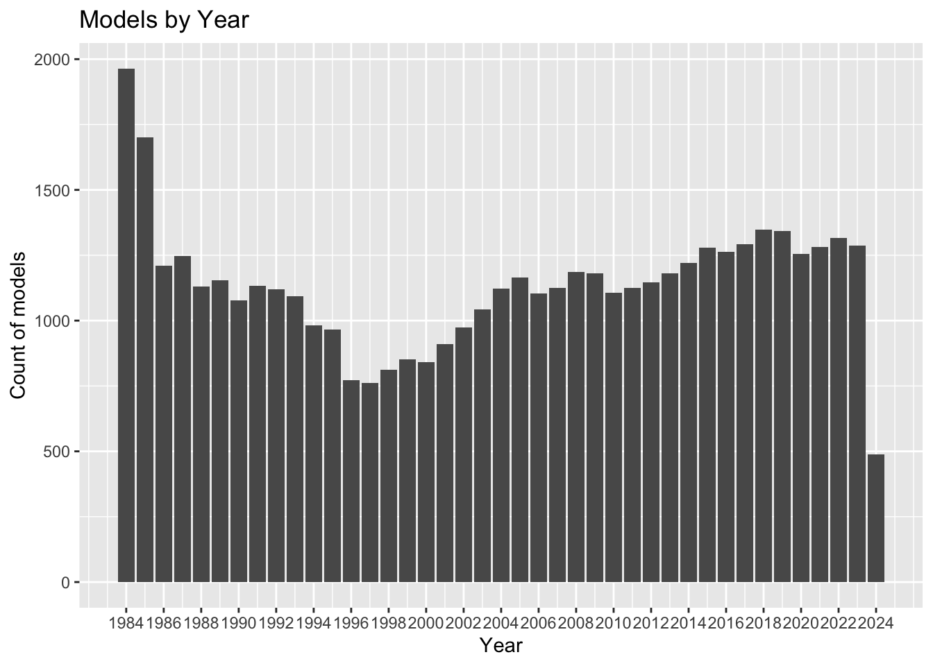
Vehicles and Years
How many models are released per year?
# Add some extra information for later use
vehicles <- vehicles %>%
  mutate(fuelType_f = gsub(fuelType1, pattern = regex('.*Gasoline', ignore_case = TRUE), replacement = 'Gasoline'))

current_model_year <- max(vehicles$year)

vehicles %>%
  ggplot(aes(x=year)) +
  geom_bar( aes(fill = year), stat = "count", show.legend = FALSE) +
  labs(title = "Models by Year", y = "Count of models", x = "Year") +
  scale_x_continuous(breaks =  seq( min(vehicles$year), max(vehicles$year), by = 2) )
Vehicles and Manufacturers
How many manufacturers do we have? We have 143 total number of manufacturers in our list. Here are the top 20.
vehicles %>%
  count(make) %>%
  top_n(20, wt = n ) %>%


  ggplot(aes(x = reorder(make, n), y = n )) +
  geom_bar( aes(fill = make), stat = "identity", show.legend = FALSE) +
    labs(title = "Top manufacturers by number of models", y = "Count of models", x = "Make") +
  coord_flip()
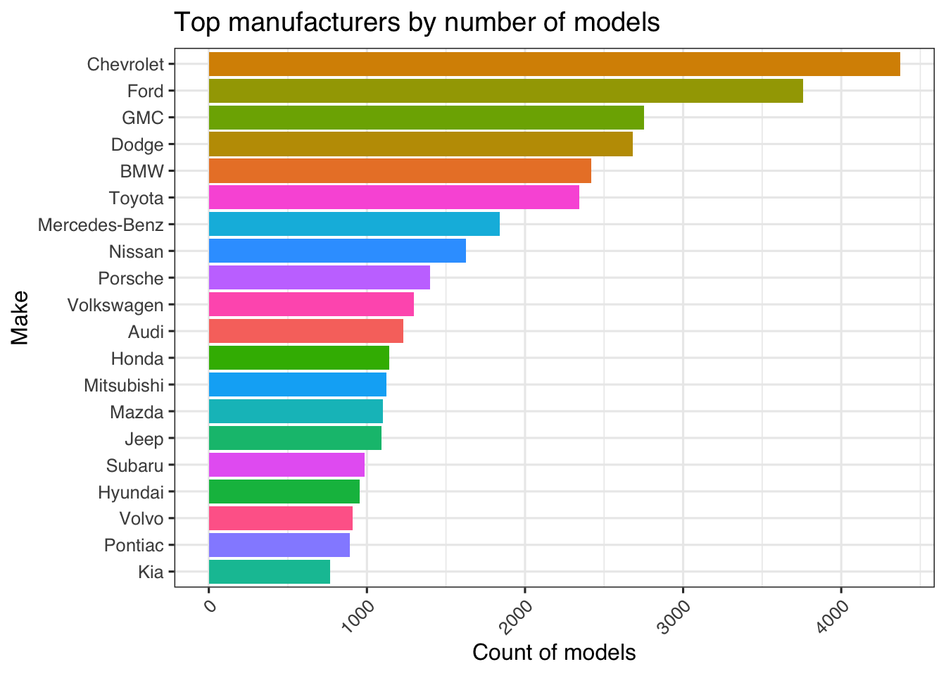
WTF, Chevrolet has close to 4000 models - this is not a real number because each manufacturer (make) has the same model coming back in a different year. We will need to identify truly unique models.
vehicles %>%
  count(make, model) %>% count(make) %>% top_n(20, wt = n) %>%
  ggplot(aes(x = reorder(make, n), y = n )) +
  geom_bar( aes(fill = make), stat = "identity", show.legend = FALSE) +
    labs(title = "Top manufacturers by number of models - adjusted for model year", y = "Count of models", x = "Make") +
  coord_flip()
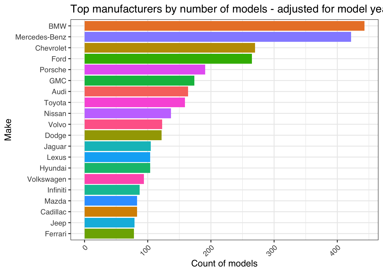
This looks a lot better - Mercedes and BMW are the most prolific manufacturers with over 300 models.
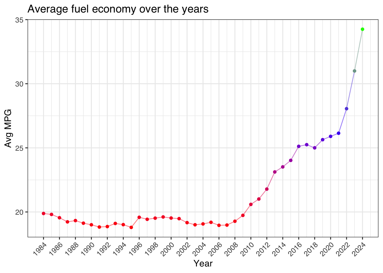
Fuel Economy
Let’s dive into an analysis of fuel economy and see how things have changed over the year, clearly economy has gone up but seems to have suffered recently. We will try and investigate why that happened. The other issue is that this data contains other types of alternative fuels, we need to adjust for different fuel types.
vehicles %>%
  group_by(year) %>%
  summarise(avgMPG = mean(comb08)) %>%
  ggplot(aes(x=year, y = avgMPG)) +
  geom_line(aes(color = avgMPG), alpha = 0.5, show.legend = FALSE) +
  geom_point(aes(color = avgMPG), show.legend = FALSE) +
  scale_x_continuous(breaks =  seq( min(vehicles$year), max(vehicles$year), by = 2) ) +
  scale_color_gradientn(colours=c("red", "blue", "green")) +
  labs(title = "Average fuel economy over the years", y = "Avg MPG", x = "Year")
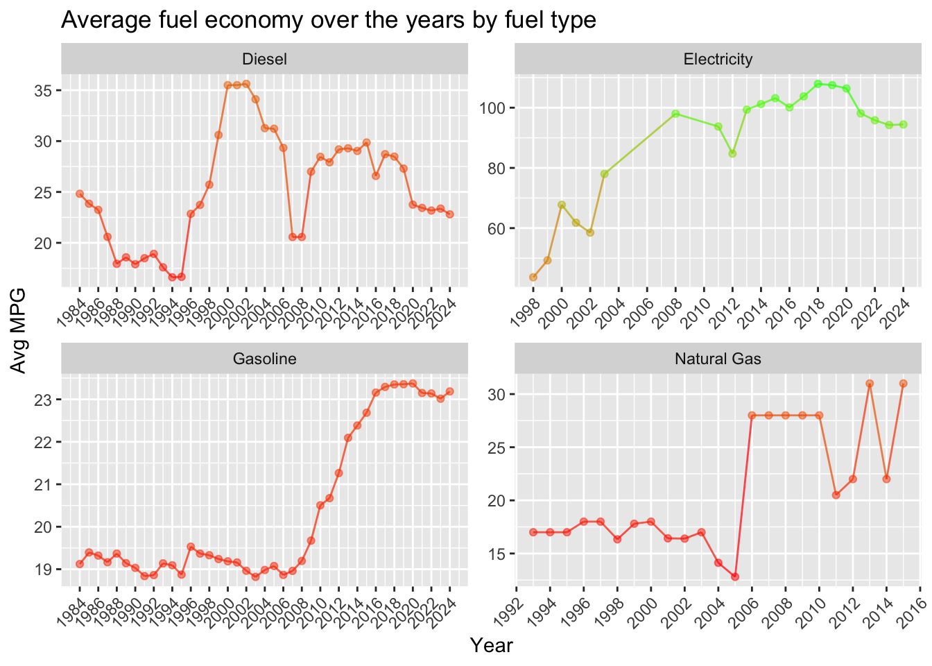
By Fuel type
Let’s look at the vehicles by the type of fuel - we had previously added an additional column that describes the different fuel types for these vehicles. Clearly, electric powered vehicles have an edge over other forms of fuel.
vehicles %>%
  group_by(year, fuelType_f) %>%
  summarise(avgMPG = mean(comb08), .groups = "drop") %>%
  ggplot(aes(x=year, y = avgMPG)) +
  geom_line(aes(color = avgMPG), alpha = 0.7, show.legend = FALSE) +
  geom_point(aes(color = avgMPG), alpha = 0.5, show.legend = FALSE) +
  scale_x_continuous(breaks =  seq( min(vehicles$year), max(vehicles$year), by = 2) ) +
  scale_color_gradientn(colours=c("red", "green")) +
  labs(title = "Average fuel economy over the years by fuel type", y = "Avg MPG", x = "Year") +
  facet_wrap(~ fuelType_f, scales = "free") +
  theme(axis.text.x = element_text(angle = 45, vjust = 1, hjust = 1), legend.direction = "horizontal", legend.position = "top")
By Vehicle class
For this we will limit ourselves to Gasoline fueled vehicles since not all vehicles are made equal, let’s also try and see how different vehicle classes score.
vehicles %>%
  filter(fuelType_f == 'Gasoline') %>%
  group_by(year, VClass) %>%
  summarise(avgMPG = mean(comb08)) %>%
  ggplot() +
  ggridges::geom_density_ridges(aes(x = avgMPG, y = as.factor(VClass), fill = VClass), rel_min_height = 0.001, scale = 1, show.legend = FALSE) +
  labs(title = "Fuel economy density by Vehicle class", y = "Vehicle Class", x = "Avg MPG")
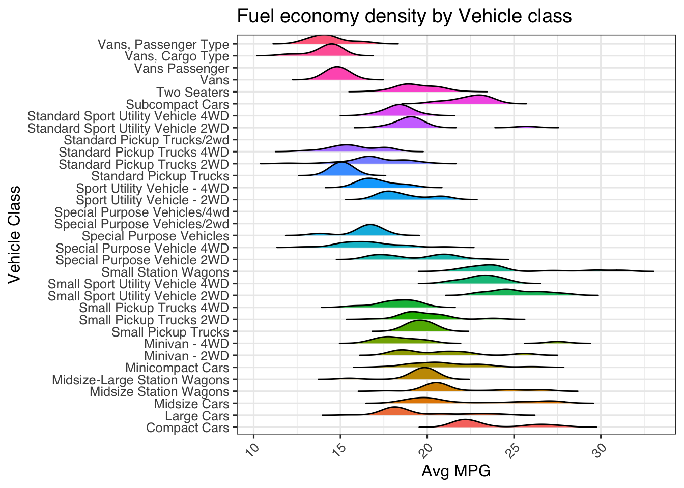
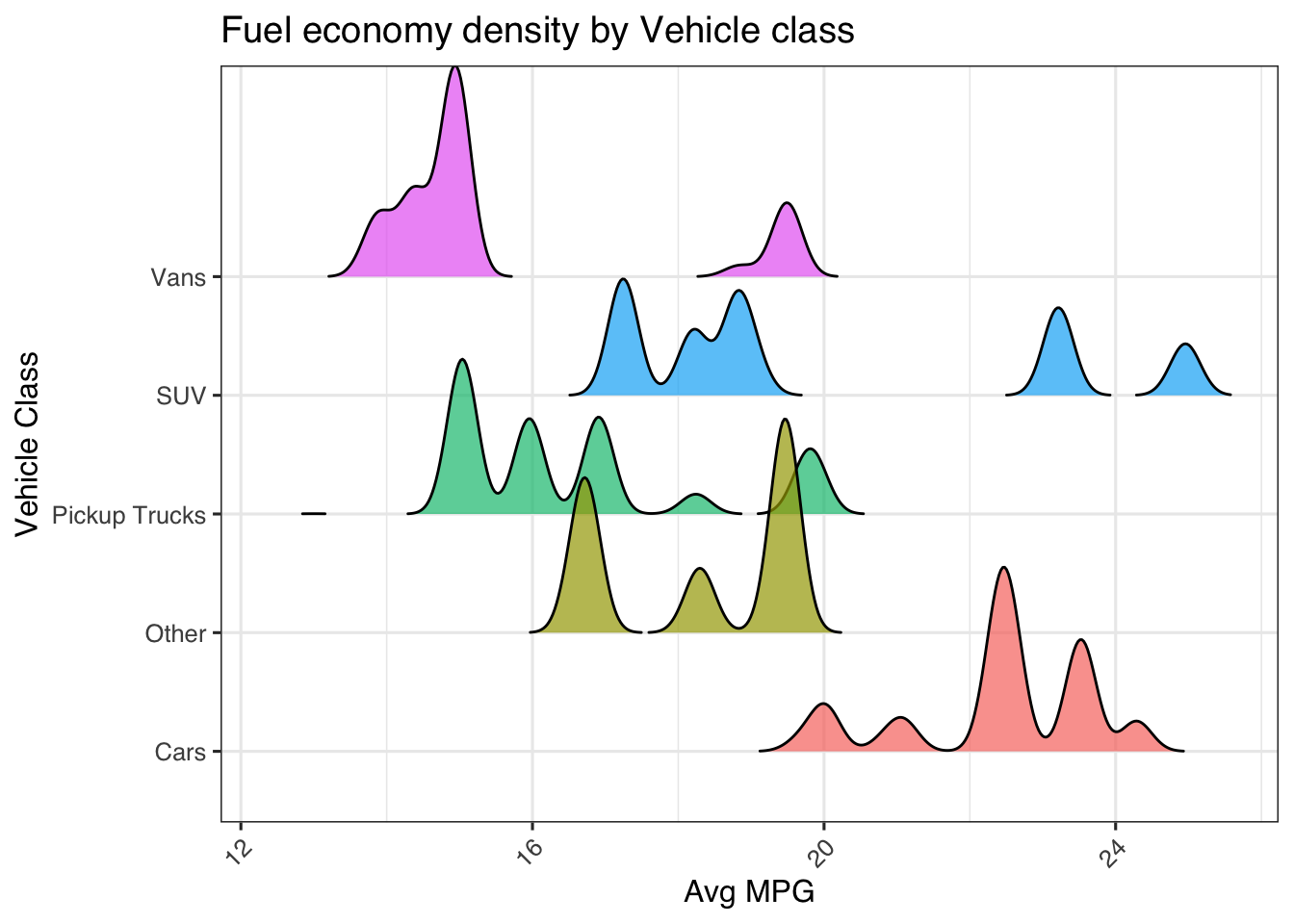
It’s clear that we are comparing apples to oranges - let’s roll up the data to create some vehicle classes and try this again.
vehicles <- vehicles %>%
  mutate(VClass_f = case_when(str_detect(VClass, pattern = "Trucks") ~ "Pickup Trucks",
                              str_detect(VClass, pattern = "Cars|Wagons") ~ "Cars",
                              str_detect(VClass, pattern = "Sport") ~ "SUV",
                              str_detect(VClass, pattern = regex("van", ignore_case = TRUE) ) ~ "Vans",
                              TRUE ~ "Other"))
We can start to see the range of mpg averages over the different vehicle classes. This graph represents the density (relative proportions) of mpg ratings in each vehicle class.
vehicles %>%
  filter(fuelType_f == 'Gasoline' , fuelType2 != "Electricity") %>%
  group_by( VClass) %>%
  mutate(avgMPG = mean(comb08)) %>% ungroup() %>%
  ggplot(aes(x = avgMPG, y = as.factor(VClass_f))) +
  geom_density_ridges(aes(fill = VClass_f), rel_min_height = 0.001, show.legend = FALSE, alpha = 0.7) +
  labs(title = "Fuel economy density by Vehicle class", y = "Vehicle Class", x = "Avg MPG")
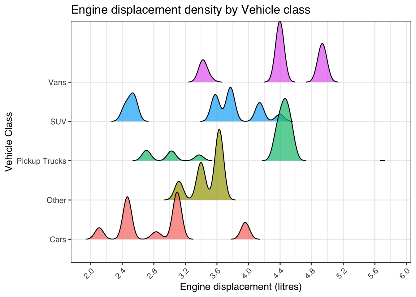
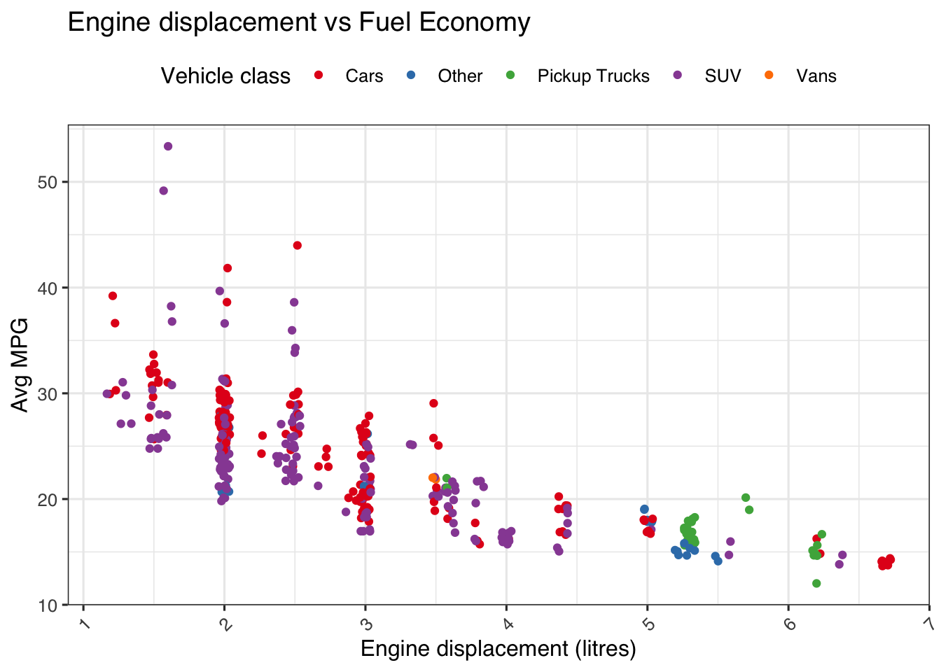
Let’s see what kind of engine displacements we are talking about in this set. It’s clear that there is a correlation between displacement and fuel economy. We will explore that later.
vehicles %>%
  filter(fuelType_f == 'Gasoline', fuelType2 != "Electricity") %>%
  group_by( VClass) %>%
  mutate(avgDispl = mean(displ)) %>% ungroup() %>%
  ggplot(aes(x = avgDispl, y = as.factor(VClass_f))) +
  geom_density_ridges(aes(fill = VClass_f), rel_min_height = 0.001, show.legend = FALSE, alpha = 0.7) +
  labs(title = "Engine displacement density by Vehicle class", y = "Vehicle Class", x = "Engine displacement (litres)") +
  scale_x_continuous(breaks = seq(1.6,6, by = 0.4))
Engine displacement vs fuel economy
- Not including plug-in hybrids.
vehicles %>%
  filter(fuelType_f == 'Gasoline' , fuelType2 != "Electricity", year == current_model_year) %>%
  ggplot(aes(y=comb08, x = displ)) +
  geom_point(aes(color = VClass_f, group = VClass_f), position = "jitter",  na.rm = TRUE ) +
  scale_color_brewer(palette = "Set1") +
  labs(title = "Engine displacement vs Fuel Economy", y = "Avg MPG", x = "Engine displacement (litres)") +
  guides(color = guide_legend(title="Vehicle class"))
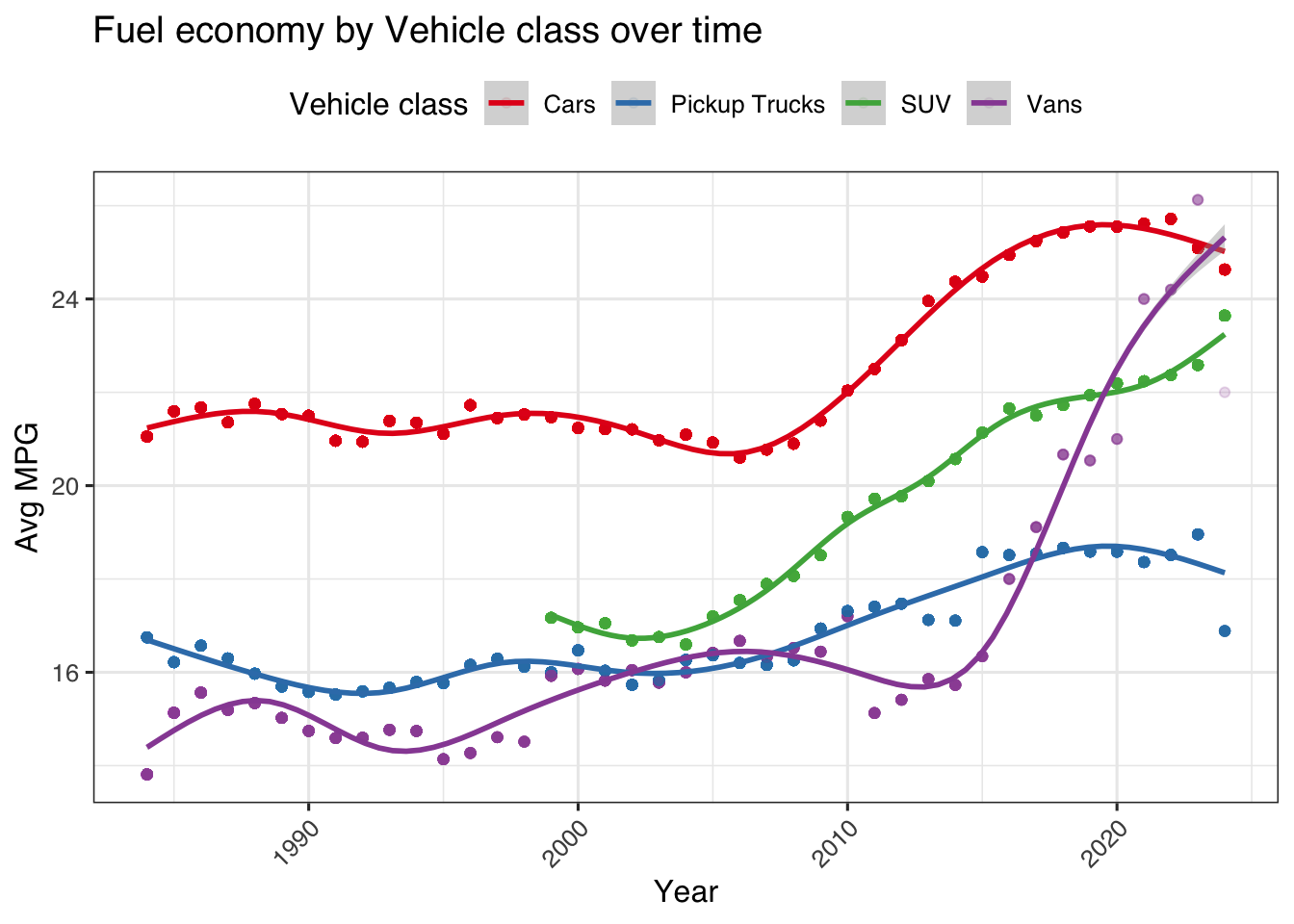
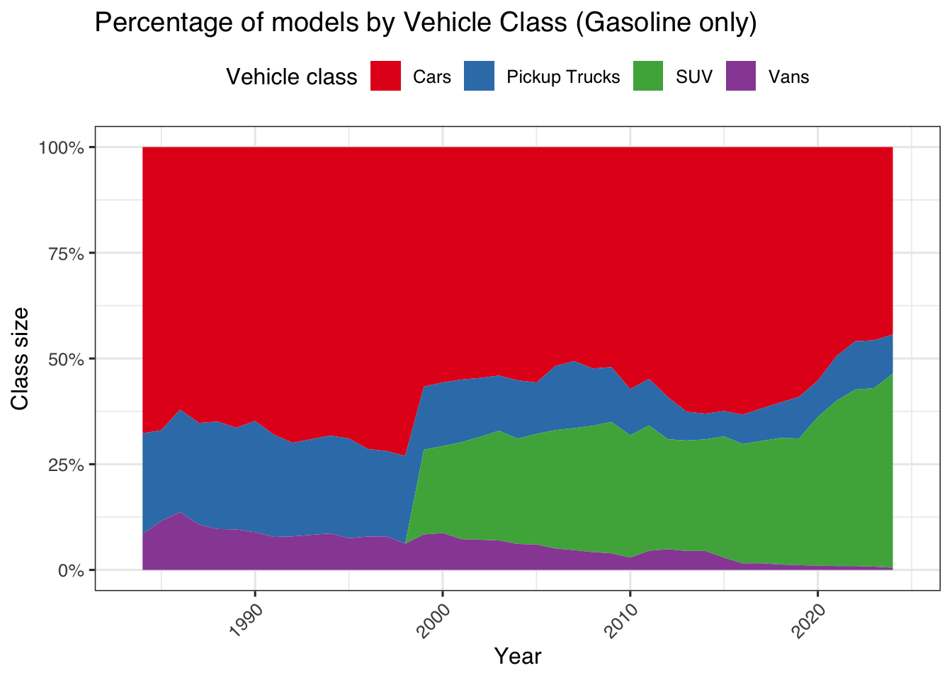
Let’s also see how has economy improved over the years for each of these segments; cars and Vans have had the most improvement over time and SUVs are a relatively new segment and were only defined near 2000. The second chart shows the relative numbers of models in each class.
vehicles %>%
  filter(fuelType_f == 'Gasoline',VClass_f != "Other") %>%
  group_by(year, VClass_f) %>%
  mutate(avgMPG = mean(comb08)) %>%
  ungroup() %>%
  ggplot(aes(x = year, y = avgMPG)) +
  geom_point(aes(color = VClass_f), alpha = 0.1) +
  geom_smooth(aes(color = VClass_f))  +
  labs(title = "Fuel economy by Vehicle class over time", y = "Avg MPG", x = "Year") +
  guides(color = guide_legend(title="Vehicle class")) +
  scale_color_brewer(palette = "Set1")
vehicles %>%
  filter(fuelType_f == 'Gasoline',VClass_f != "Other") %>%
  group_by(year, VClass_f) %>%
  ungroup() %>%
  ggplot(aes(x = year, y = ..count..)) +
  geom_area(aes(fill = VClass_f), stat= "bin", position = "fill", binwidth = 1) +
  labs(title = "Percentage of models by Vehicle Class (Gasoline only)", y = "Class size", x = "Year") +
  guides(fill = guide_legend(title="Vehicle class")) +
  scale_y_continuous(labels = scales::percent, breaks = seq(0,1, by = .25)) +
  scale_fill_brewer(palette = "Set1")
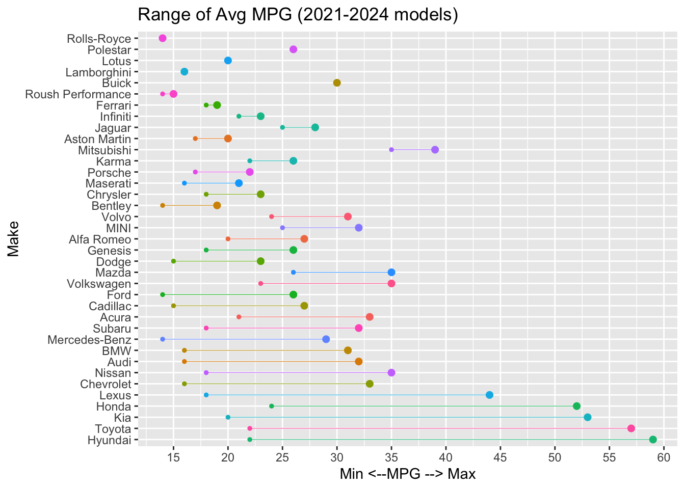
By manufacturers
Are there manufacturers that have done a better job compared to the others? Let’s start by seeing what the range of mileage is in our data set, still only looking at the Gasoline segment only. Let’s do this for the last three model years only. We can see a wide swing in range between different models from a manufacturer. Hyundai seems quite curious with a range from 17 to 58 mpg, we’ll try and explore that further.
vehicles %>%
  filter(fuelType_f == 'Gasoline',VClass_f == "Cars", between(year, current_model_year-3, current_model_year)) %>%
  group_by(make) %>%
  summarise(min = min(comb08), max = max(comb08)) %>%

  ggplot() +
    geom_point(aes(x = reorder(make, -(max - min), order = TRUE ), y = max, color = make), size = 2, show.legend = FALSE)  +
    geom_point(aes(x = make, y = min, color = make), size = 1, show.legend = FALSE) +
    geom_segment(aes(x = make, xend = make, y = min, yend = max, color = make), linewidth = 0.2, show.legend = FALSE) +
    coord_flip() +
    scale_y_continuous(breaks = seq(10,60, by = 5)) +
    labs(title = paste0("Range of Avg MPG (", current_model_year -3, "-", current_model_year, " models)"), x = "Make", y = "Min <--MPG --> Max")
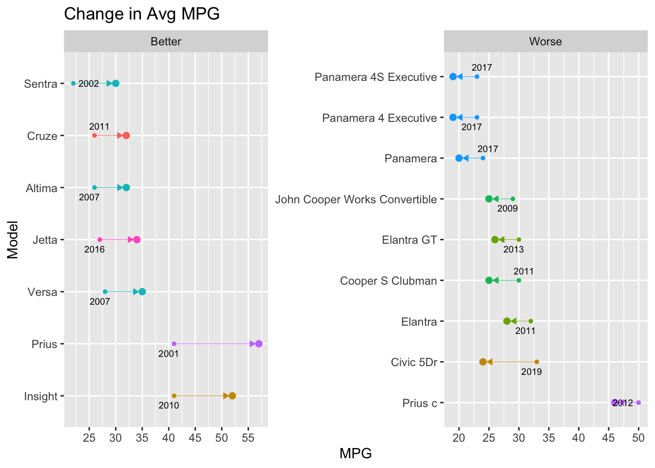
Most Improved
My goal here is to find the most fuel efficient vehicles. There are many ways to slice this data to find the best vehicles; by make, by vehicle class, by fuel type, by engine size, seating capacity and many other ways. One interesting metric would be to see which models have the most improved efficiency over time. We will find vehicles that are still being sold in the current model year and have been around for at least three model years. Once more, we’ll limit our set to Gasoline powered vehicles only. The chart below shows the most improved and ones that have gotten much worse over the years.
# Find models that are still being sold in the current model year
vehicles %>%
  filter(year == 2019, fuelType_f == "Gasoline", VClass_f == "Cars") %>%
  distinct(make, model, fuelType_f, trany, fuelType, cylinders) %>%
  inner_join(vehicles, by = c("make", "model", "trany", "fuelType", "cylinders")) %>%
  group_by(make, model, trany, fuelType, cylinders) %>%
  summarise(years_sold = n_distinct(year), mpg_start = comb08[which.min(year)], mpg_end = comb08[which.max(year)], mpg_range = mpg_end - mpg_start, min_year = year[which.min(year)], max_year = year[which.max(year)], .groups = "drop") %>%
  mutate(avg_range = mean(mpg_range), sd_range = sd(mpg_range), shift = if_else(mpg_range > 0, "Better", "Worse")) %>%
  filter(years_sold > 2, mpg_range > 3 * sd_range | mpg_range < -2* sd_range) %>%

  ggplot() +
    geom_point(aes(x = reorder(model, -mpg_start), y = mpg_end, color = make), size = 2, show.legend = FALSE) +
    geom_point(aes(x = model, y = mpg_start, color = make), size = 1 , show.legend = FALSE) +
    geom_segment(aes(x = model, xend = model, y = mpg_start, yend = if_else(shift == "Better", mpg_end -0.65, mpg_end + 0.65), color = make), linejoin = "mitre", arrow = arrow(length = unit(0.03, "npc"), type = "closed"), size = 0.2, show.legend = FALSE) +
    geom_text_repel(aes(x = model, y = mpg_start, label = min_year), size = 2.5 ) +
    scale_y_continuous(breaks = seq(10,60, by = 5)) +
    labs(title ="Change in Avg MPG", x = "Model", y = "MPG") +
    facet_wrap(~shift, scales = "free") +
  coord_flip()
## Warning: Using `size` aesthetic for lines was deprecated in ggplot2 3.4.0.
## ℹ Please use `linewidth` instead.
## This warning is displayed once every 8 hours.
## Call `lifecycle::last_lifecycle_warnings()` to see where this warning was
## generated.
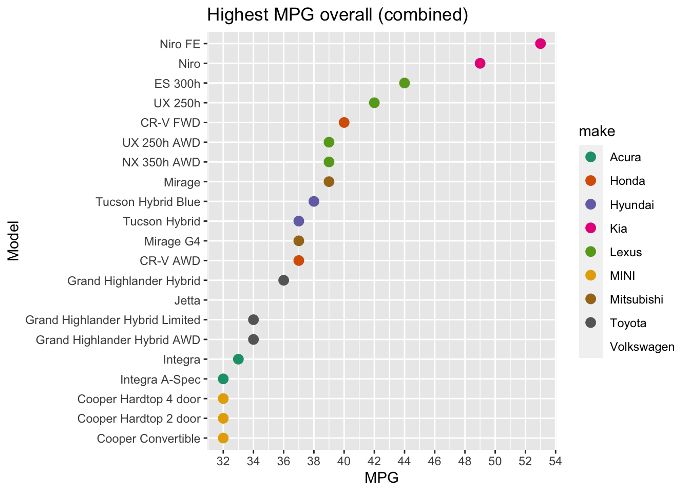
Most fuel efficient Models in class
Let’s look at the real fuel sippers by class of vehicle - we’ll start by the larger class and then refine further into smaller sub-classes. All these are the most recent models and all are Gasoline powered. We will look at other fuel types separately.
By Vehicle class
vehicles %>%
  filter(year == current_model_year, fuelType_f == "Gasoline") %>%
  top_n(20, wt = comb08) %>%
  ggplot() +
  geom_point(aes(x = reorder(model, comb08), y = comb08, color = make), size = 3) +

  coord_flip() +
  labs(title ="Highest MPG overall (combined)", x = "Model", y = "MPG") +
  scale_y_continuous(breaks = seq(30,60, by = 2)) +
  scale_color_brewer(palette = "Dark2")
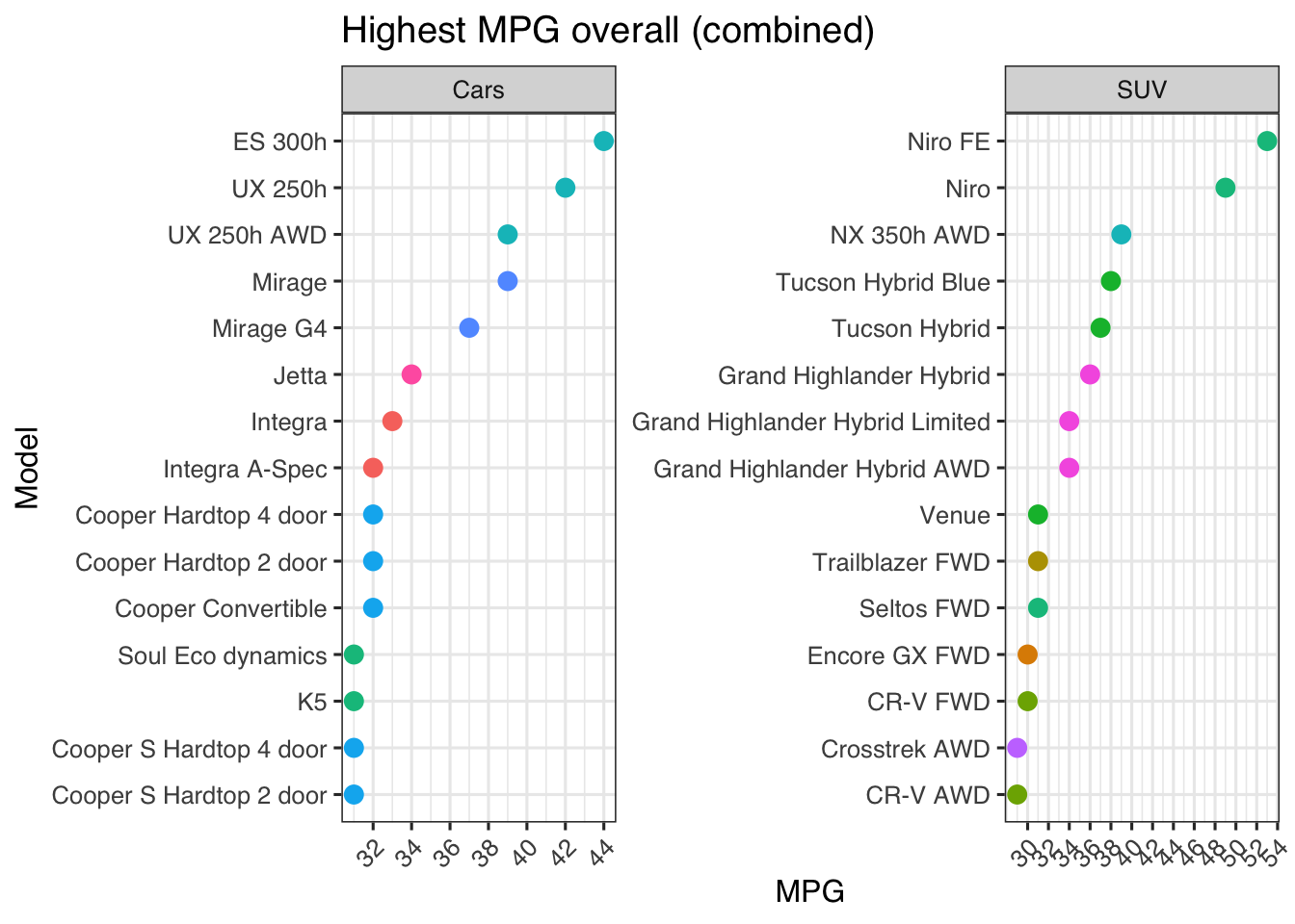
By Vehicle type
Since SUVs and Cars are the biggest segments - let’s limit to those. Only look for full gasoline or hybrid vehicles, exclude any plug in hybrids
vehicles %>%
  filter(year == current_model_year, fuelType_f == "Gasoline", fuelType2 != "Electricity", VClass_f %in% c("Cars", "SUV")) %>%
  group_by(VClass_f) %>%
  distinct(model, .keep_all = TRUE) %>%
  top_n(15, wt = comb08) %>%
  ggplot() +
  geom_point(aes(x = reorder(model, comb08), y = comb08, color = make), size = 3, show.legend = FALSE) +

  coord_flip() +
  labs(title ="Highest MPG overall (combined)", x = "Model", y = "MPG") +
  scale_y_continuous(breaks = seq(30,60, by = 2)) +
  #scale_color_brewer(palette = "Dark2") +
  facet_wrap(~ VClass_f, scales ="free")
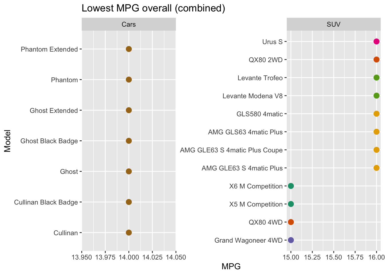
Before we move on, let’s take a quick look at the worst overall MPG
Worst MPG
Gasoline Cars - current model year Looking at this, at least Rolls Royce is constiently bad across most of it’s models and Grand Cherokee Trackhawk is a 800 bhp, 0 - 60 in less than 3 second beast.
vehicles %>%
  filter(year == current_model_year, fuelType_f == "Gasoline", fuelType2 != "Electricity", VClass_f %in% c("Cars", "SUV")) %>%
  group_by(VClass_f) %>%
  distinct(model, .keep_all = TRUE) %>%
  top_n(5, wt = -comb08) %>%
  ggplot() +
  geom_point(aes(x = reorder(model, comb08), y = comb08, color = make), size = 3, show.legend = FALSE) +

  coord_flip() +
  labs(title ="Lowest MPG overall (combined)", x = "Model", y = "MPG") +
  #scale_y_continuous(breaks = seq(10,18, by = 2)) +
  scale_color_brewer(palette = "Dark2") +
  facet_wrap(~ VClass_f, scales ="free")
Electric Vehicles
Before looking at the data, a quick look a the number of models for each fuel type
Different Fuel Types
- Current model year only
vehicles %>%
  filter(year == current_model_year, VClass_f != "Other") %>%
  group_by(fuelType_f) %>%
  ggplot(aes( x = fuelType_f)) +
  geom_bar(aes(fill = fuelType_f)) +
  scale_fill_brewer(palette = "Set1") +
  facet_grid(~ VClass_f, scales = "free") +
  labs(title = "Count of models by fuel type - Current model year", y = "Class size", x = "Fuel Type") +
  guides(fill = guide_legend(title="Vehicle class")) +
  geom_label(stat = "count", aes(label = ..count.., y = ..count..)) +
  theme(axis.text.x = element_text(angle = 45, vjust = 1, hjust = 1), legend.direction = "horizontal", legend.position = "top")
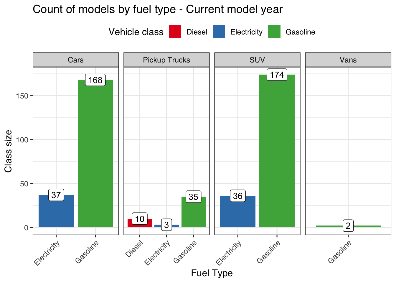
While EVs are still an extremely small segment of the total passenger vehicle segment, they are certainly starting to be noticed. Let’s look at the electric vehicle stats before we move to some machine learning.
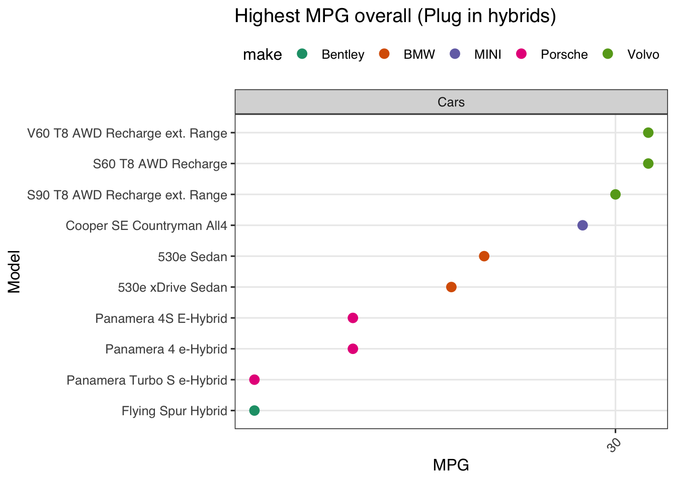
Electric Effciency
We’ll look at the transitional electric vehicles first - these are also called the plug-in electric vehicles where they retain an IC engine along with some battery.
vehicles %>%
  filter(fuelType2 == "Electricity", year == current_model_year -1, VClass_f %in% c("Cars")) %>%
  group_by(VClass_f) %>%
  distinct(model, .keep_all = TRUE) %>%
  top_n(15, wt = comb08) %>%
  ggplot() +
  geom_point(aes(x = reorder(model, comb08), y = comb08, color = make), size = 3) +

  coord_flip() +
  labs(title ="Highest MPG overall (Plug in hybrids)", x = "Model", y = "MPG") +
  scale_y_continuous(breaks = seq(30,60, by = 2)) +
  scale_color_brewer(palette = "Dark2") +
  facet_wrap(~ VClass_f, scales ="free")
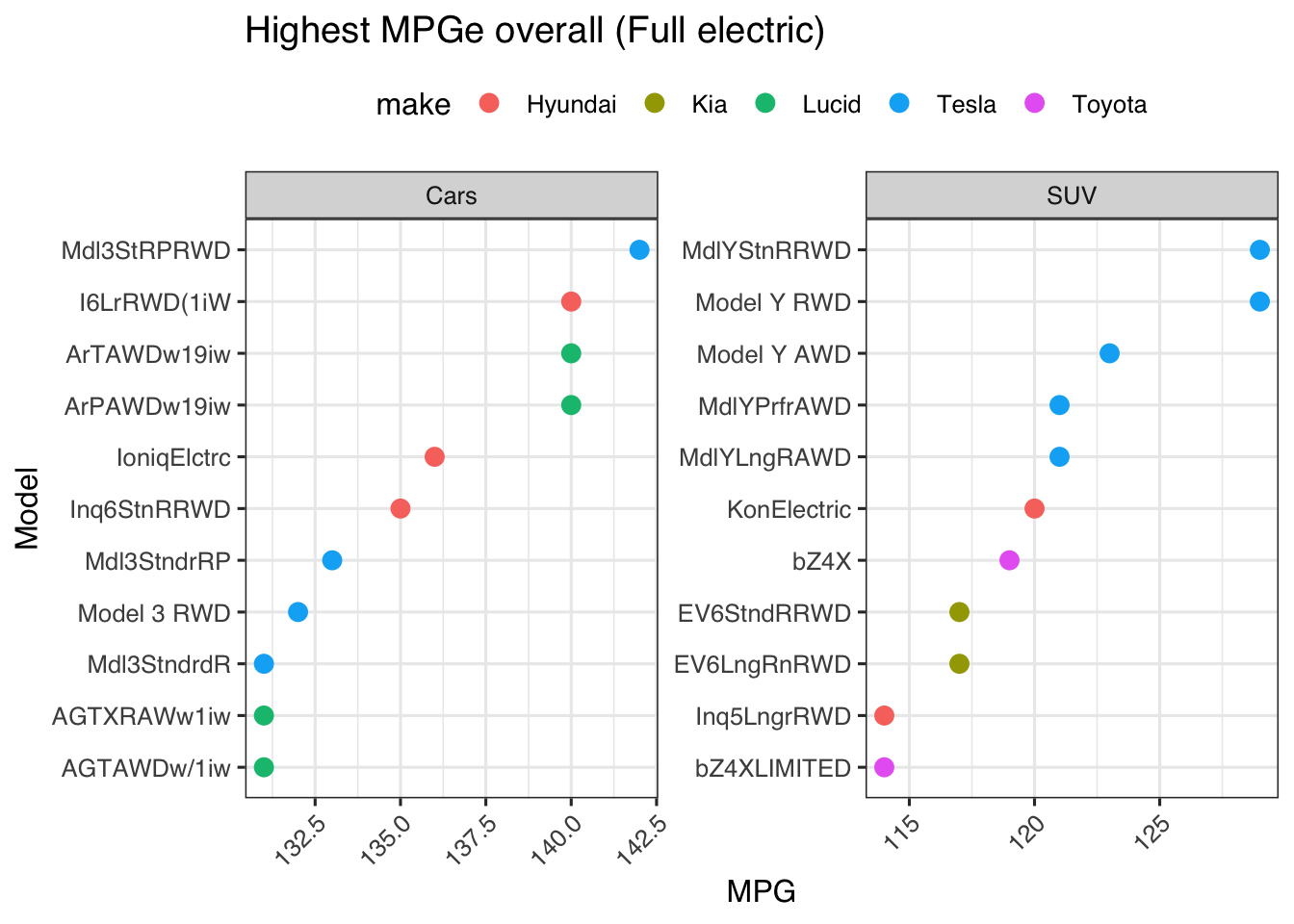
Fully electric
Hyundai seems to have taken the top spots in both the Cars and SUV segments and Tesla is doing well in both segments.
vehicles %>%
  filter(fuelType_f == "Electricity",  VClass_f %in% c("Cars", "SUV")) %>%
  group_by(VClass_f) %>%
  distinct(model, .keep_all = TRUE) %>%
  top_n(10, wt = comb08) %>%
  ggplot() +
  geom_point(aes(x = reorder(model, comb08), y = comb08, color = make), size = 3) +

  coord_flip() +
  labs(title ="Highest MPGe overall (Full electric)", x = "Model", y = "MPG") +
  facet_wrap(~ VClass_f, scales ="free") +
  scale_x_discrete(labels = function(x) abbreviate(x, minlength = 11L))
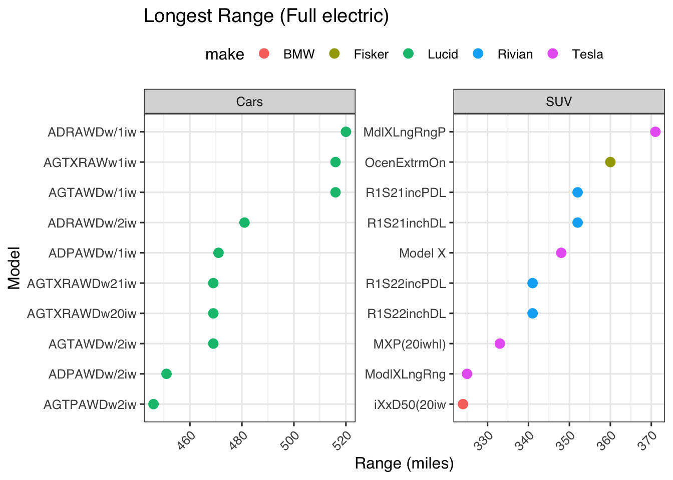
Fully electric range
What kind of range do we get at the top of the heap and it’s clear that Tesla has done a phenomenal job both in efficiency and range.
vehicles %>%
  filter(fuelType_f == "Electricity", VClass_f %in% c("Cars", "SUV")) %>%
  group_by(VClass_f) %>%
  distinct(model, .keep_all = TRUE) %>%
  top_n(10, wt = range) %>%
  ggplot() +
  geom_point(aes(x = reorder(model, range), y = range, color = make), size = 3) +

  coord_flip() +
  labs(title ="Longest Range (Full electric)", x = "Model", y = "Range (miles)") +
  facet_wrap(~ VClass_f, scales ="free") +
  scale_x_discrete(labels = function(x) abbreviate(x, minlength = 11L))
Machine Learning
This is a great dataset to try and dig into machine learning. Start with some clustering
Clustering
Clustering is process of grouping together similar items. In this case we want to see which vehicles are most like another and form groups.
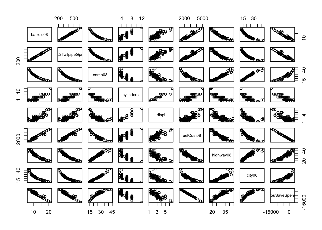
Before we get into the actual clustering, we’ll try and identify which variables are related and which are ones that are important. We’ll use a technique called Principal Component Analysis. Let’s take a look at what the data looks like; some of these are clearly propotinally and linearly related, while others have some more spread out variations.
data <- vehicles %>%
  filter(year == current_model_year, fuelType_f == "Gasoline", fuelType2 != "Electricity",  VClass_f == "Cars") %>%
  distinct( model,  trany,  cylinders, .keep_all = TRUE) %>%
  mutate(model = paste(model, trany, cylinders, sep = "-")) %>%
  select(model, barrels08, co2TailpipeGpm, comb08, cylinders, displ, fuelCost08, highway08, city08, youSaveSpend)

data <- na.omit(data)
data <- as.data.frame(data)
rownames(data) <- data$model
data <- select(data, -model)

plot(data)
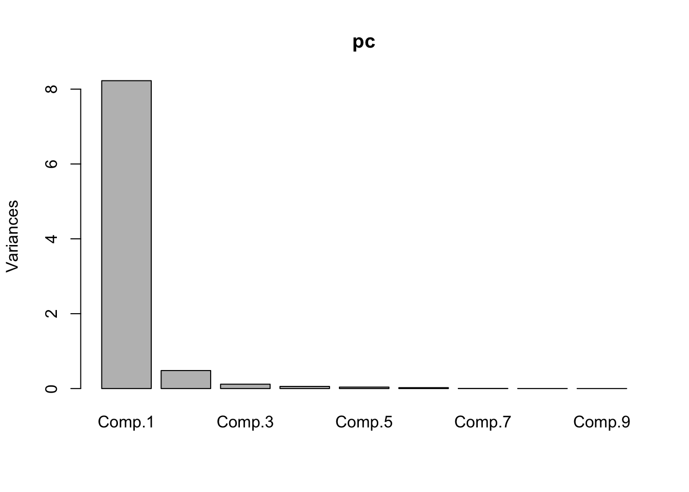
Before we run the principal components, we’ll scale the data to normalize it - that will ensure that the data ranges are normalized and one single element does not have a large range and does not dominate.
df <- scale(data)
pc <- princomp(df)
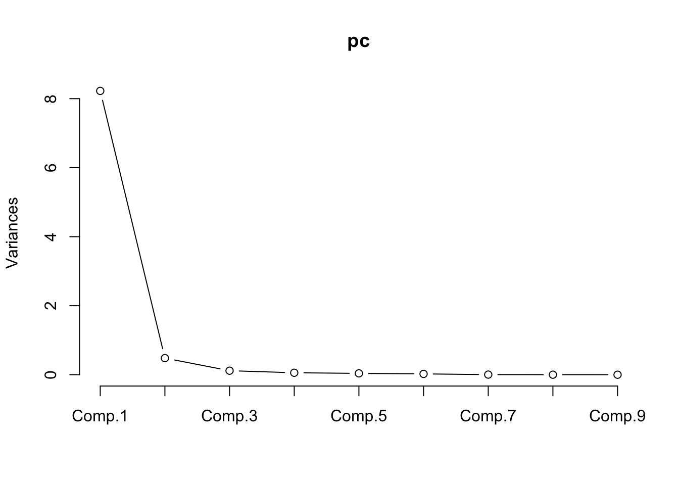
plot(pc)
plot(pc, type='l')
summary(pc)
## Importance of components:
##                           Comp.1     Comp.2     Comp.3     Comp.4      Comp.5
## Standard deviation     2.8679524 0.69353668 0.34128805 0.23797680 0.196730951
## Proportion of Variance 0.9194782 0.05376956 0.01302086 0.00633092 0.004326562
## Cumulative Proportion  0.9194782 0.97324778 0.98626865 0.99259957 0.996926128
##                            Comp.6       Comp.7       Comp.8       Comp.9
## Standard deviation     0.15390415 0.0565386169 2.478054e-02 9.684188e-09
## Proportion of Variance 0.00264788 0.0003573452 6.864661e-05 1.048393e-17
## Cumulative Proportion  0.99957401 0.9999313534 1.000000e+00 1.000000e+00
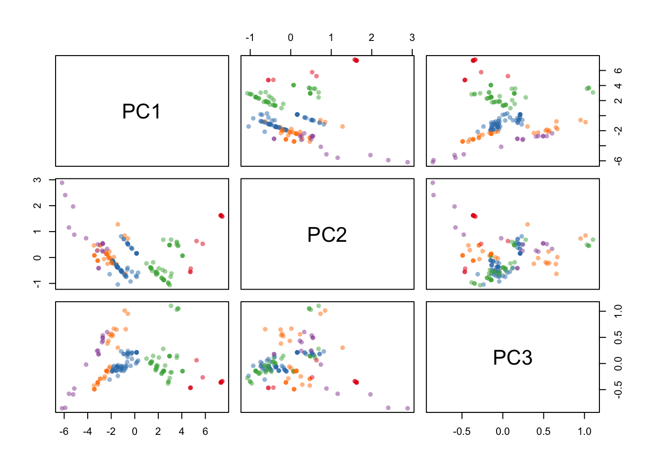
Given these charts, we will use the first three components from this data since most variation is present in these three. We have now simplified the data into fewer dimensions that have the most variance and are therefore the most important in deciding clusters. The columns we have selected are barrels08, co2TailpipeGpm, comb08
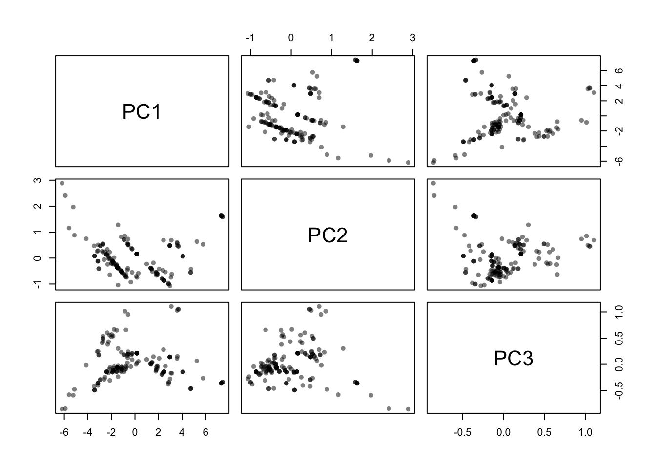
pc <- prcomp(df)
comp <- data.frame(pc$x[,1:3])
# Plot
plot(comp, pch=16, col=rgb(0,0,0,0.5))
K-means
The k means algorithm tries to create groups of observations by minimizing the distance between the observations, the other question to answer as we do this is to find out the optimal number of clusters. A second thing to note is that since all our data has many different ranges, to compare standard measures, we’ll re-scale all the data after removing all non-numeric data.
One of the first things we need to identify is an optimum number of clusters we should seek. Here I used the code from R in Action:
# Determine number of clusters
wss <- (nrow(comp)-1)*sum(apply(comp,2,var))
for (i in 2:15) wss[i] <- sum(kmeans(comp,
                                     centers=i)$withinss)
plot(1:15, wss, type="b", xlab="Number of Clusters",
     ylab="Within groups sum of squares")
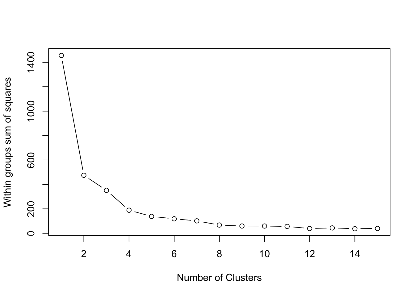
Based on the scree plot above, let’s go with 5 clusters within this data.
# Only do this for gasoline cars initially
set.seed(1215)
k <- kmeans(data, 5, nstart=25, iter.max=1000)
palette(alpha(brewer.pal(9,'Set1'), 0.5))
plot(comp, col=k$clust, pch=16)
Finally, we can identify the vehicles that have been clustered together.
clust <- names(table(k$clust))

# First cluster

map(clust, function(x) {
  row.names(data[k$clust==x,])
})
## [[1]]
##  [1] "Ghibli Trofeo-Automatic 8-spd-8"
##  [2] "Quattroporte Trofeo-Automatic 8-spd-8"
##  [3] "Urus Performante-Automatic (S8)-8"
##  [4] "CT5 V-Manual 6-spd-8"
##  [5] "CT5 V-Automatic (S10)-8"
##  [6] "Phantom-Automatic (S8)-12"
##  [7] "Phantom Extended-Automatic (S8)-12"
##  [8] "Ghost-Automatic (S8)-12"
##  [9] "Ghost Extended-Automatic (S8)-12"
## [10] "Ghost Black Badge-Automatic (S8)-12"
## [11] "Cullinan-Automatic (S8)-12"
## [12] "Cullinan Black Badge-Automatic (S8)-12"
##
## [[2]]
##  [1] "Cooper S Convertible-Manual 6-spd-4"
##  [2] "John Cooper Works Convertible-Automatic (S8)-4"
##  [3] "430i Coupe-Automatic (S8)-4"
##  [4] "430i xDrive Coupe-Automatic (S8)-4"
##  [5] "430i Convertible-Automatic (S8)-4"
##  [6] "430i xDrive Convertible-Automatic (S8)-4"
##  [7] "840i Coupe-Automatic (S8)-6"
##  [8] "840i xDrive Coupe-Automatic (S8)-6"
##  [9] "840i Convertible-Automatic (S8)-6"
## [10] "840i xDrive Convertible-Automatic (S8)-6"
## [11] "Cooper S Hardtop 2 door-Manual 6-spd-4"
## [12] "Cooper S Hardtop 4 door-Manual 6-spd-4"
## [13] "John Cooper Works Hardtop 2 door-Manual 6-spd-4"
## [14] "430i Gran Coupe-Automatic (S8)-4"
## [15] "430i xDrive Gran Coupe-Automatic (S8)-4"
## [16] "840i Gran Coupe-Automatic (S8)-6"
## [17] "840i xDrive Gran Coupe-Automatic (S8)-6"
## [18] "Cooper Countryman-Automatic (AM-S7)-3"
## [19] "Cooper Countryman All4-Automatic (S8)-3"
## [20] "John Cooper Works Clubman All4-Automatic (S8)-4"
## [21] "JCW Countryman All4-Automatic (S8)-4"
## [22] "M440i Coupe-Automatic (S8)-6"
## [23] "M440i xDrive Coupe-Automatic (S8)-6"
## [24] "M440i Convertible-Automatic (S8)-6"
## [25] "M440i xDrive Convertible-Automatic (S8)-6"
## [26] "M440i Gran Coupe-Automatic (S8)-6"
## [27] "M440i xDrive Gran Coupe-Automatic (S8)-6"
## [28] "Cooper S Clubman-Manual 6-spd-4"
## [29] "Cooper S Countryman-Automatic (AM-S7)-4"
## [30] "Cooper S Countryman All4-Automatic (S8)-4"
## [31] "Cooper S Clubman All4-Automatic (S8)-4"
## [32] "Giulia-Automatic 8-spd-4"
## [33] "Giulia AWD-Automatic 8-spd-4"
## [34] "RS 3-Automatic (AM-S7)-5"
## [35] "S3-Automatic (AM-S7)-4"
## [36] "M240i Coupe-Automatic (S8)-6"
## [37] "228i xDrive Gran Coupe-Automatic (S8)-4"
## [38] "228i Gran Coupe-Automatic (S8)-4"
## [39] "M235i xDrive Gran Coupe-Automatic (S8)-4"
## [40] "330i xDrive Sedan-Automatic (S8)-4"
## [41] "S60 B5 AWD-Automatic (S8)-4"
## [42] "XF P250-Automatic (S8)-4"
## [43] "S90 B6 AWD-Automatic (S8)-4"
## [44] "Integra-Manual 6-spd-4"
## [45] "G80 AWD-Automatic (S8)-4"
## [46] "V60CC B5 AWD-Automatic (S8)-4"
## [47] "V90CC B6 AWD-Automatic (S8)-4"
## [48] "230i xDrive Coupe-Automatic (S8)-4"
## [49] "M240i xDrive Coupe-Automatic (S8)-6"
## [50] "M340i Sedan-Automatic (S8)-6"
## [51] "M340i xDrive Sedan-Automatic (S8)-6"
## [52] "CT4-Automatic (S10)-4"
## [53] "CT4-Automatic (S8)-4"
## [54] "CT4 AWD-Automatic (S8)-4"
## [55] "CT4 AWD-Automatic (S10)-4"
## [56] "CT4 V AWD-Automatic (S10)-4"
## [57] "CT4 V-Automatic (S10)-4"
## [58] "CT5-Automatic (S10)-4"
## [59] "CT5 AWD-Automatic (S10)-4"
## [60] "740i Sedan-Automatic (S8)-6"
##
## [[3]]
##  [1] "M4 Coupe-Manual 6-spd-6"
##  [2] "M4 Competition Coupe-Automatic (S8)-6"
##  [3] "M4 Competition M xDrive Coupe-Automatic (S8)-6"
##  [4] "M4 Competition M xDrive Convertible-Automatic (S8)-6"
##  [5] "M850i xDrive Coupe-Automatic (S8)-8"
##  [6] "M850i xDrive Convertible-Automatic (S8)-8"
##  [7] "M8 Competition Coupe-Automatic (S8)-8"
##  [8] "M8 Competition Convertible-Automatic (S8)-8"
##  [9] "M850i xDrive Gran Coupe-Automatic (S8)-8"
## [10] "Alpina B8 Gran Coupe-Automatic (S8)-8"
## [11] "M8 Competition Gran Coupe-Automatic (S8)-8"
## [12] "M3 CS Sedan-Automatic (S8)-6"
## [13] "GT-R-Automatic (AM-S6)-6"
## [14] "GranTurismo Trofeo-Automatic 8-spd-6"
## [15] "GranTurismo Modena-Automatic 8-spd-6"
## [16] "LC 500 Convertible-Automatic (S10)-8"
## [17] "RS 5 Coupe-Automatic (S8)-6"
## [18] "M2 Coupe-Manual 6-spd-6"
## [19] "M2 Coupe-Automatic (S8)-6"
## [20] "Mustang-Manual 6-spd-8"
## [21] "Mustang-Automatic (S10)-8"
## [22] "Mustang Dark Horse-Manual 6-spd-8"
## [23] "LC 500-Automatic (S10)-8"
## [24] "M3 Sedan-Manual 6-spd-6"
## [25] "M3 Competition Sedan-Automatic (S8)-6"
## [26] "M3 Competition M xDrive Sedan-Automatic (S8)-6"
## [27] "RS 5 Sportback-Automatic (S8)-6"
## [28] "Ghibli GT-Automatic 8-spd-6"
## [29] "Ghibli Modena RWD-Automatic 8-spd-6"
## [30] "G80 AWD-Automatic (S8)-6"
## [31] "G90 AWD-Automatic (S8)-6"
## [32] "G90 MHEV-Automatic (S8)-6"
## [33] "Quattroporte Modena AWD-Automatic 8-spd-6"
## [34] "Quattroporte Modena RWD-Automatic 8-spd-6"
## [35] "Quattroporte GT-Automatic 8-spd-6"
## [36] "911 Carrera T-Manual 7-spd-6"
## [37] "911 Carrera T-Automatic (AM-S8)-6"
## [38] "Mustang Dark Horse-Automatic (S10)-8"
## [39] "CT4 V-Automatic (S10)-6"
## [40] "CT4 V-Manual 6-spd-6"
## [41] "Giulia-Automatic 8-spd-6"
## [42] "CT5 AWD-Automatic (S10)-6"
## [43] "CT5 V AWD-Automatic (S10)-6"
## [44] "CT5-Automatic (S10)-6"
## [45] "CT5 V-Automatic (S10)-6"
## [46] "760i xDrive Sedan-Automatic (S8)-8"
##
## [[4]]
##  [1] "Trax-Automatic 6-spd-3"
##  [2] "Legacy AWD-Automatic (AV-S8)-4"
##  [3] "Impreza-Automatic (AV-S8)-4"
##  [4] "UX 250h-Automatic (AV-S6)-4"
##  [5] "UX 250h AWD-Automatic (AV-S6)-4"
##  [6] "K5-Automatic (S8)-4"
##  [7] "Envista-Automatic 6-spd-3"
##  [8] "Mirage-Automatic (variable gear ratios)-3"
##  [9] "Mirage G4-Automatic (variable gear ratios)-3"
## [10] "Jetta-Manual 6-spd-4"
## [11] "ES 300h-Automatic (AV-S6)-4"
## [12] "3 5-Door 2WD-Manual 6-spd-4"
## [13] "3 5-Door 2WD-Automatic (S6)-4"
## [14] "3 5-Door 4WD-Automatic (S6)-4"
## [15] "Soul-Automatic (variable gear ratios)-4"
## [16] "Soul Eco dynamics-Automatic (variable gear ratios)-4"
##
## [[5]]
##  [1] "Cooper Convertible-Automatic (AM-S7)-3"
##  [2] "Cooper Convertible-Manual 6-spd-3"
##  [3] "Cooper S Convertible-Automatic (AM-S7)-4"
##  [4] "Cooper Hardtop 2 door-Automatic (AM-S7)-3"
##  [5] "Cooper Hardtop 2 door-Manual 6-spd-3"
##  [6] "Cooper Hardtop 4 door-Automatic (AM-S7)-3"
##  [7] "Cooper Hardtop 4 door-Manual 6-spd-3"
##  [8] "Cooper S Hardtop 2 door-Automatic (AM-S7)-4"
##  [9] "Cooper S Hardtop 4 door-Automatic (AM-S7)-4"
## [10] "John Cooper Works Hardtop 2 door-Automatic (S8)-4"
## [11] "Cooper S Clubman-Automatic (AM-S7)-4"
## [12] "Integra-Automatic (AV-S7)-4"
## [13] "Integra A-Spec-Automatic (AV-S7)-4"
## [14] "Integra A-Spec-Manual 6-spd-4"
## [15] "K5 AWD-Automatic (S8)-4"
## [16] "K5-Automatic (AM-S8)-4"
## [17] "HR-V AWD-Automatic (variable gear ratios)-4"
## [18] "HR-V FWD-Automatic (variable gear ratios)-4"
## [19] "230i Coupe-Automatic (S8)-4"
## [20] "Mustang Performance Package-Automatic (S10)-4"
## [21] "Mustang-Automatic 10-spd-4"
## [22] "LC 500h-Automatic (AV-S10)-6"
## [23] "A4 quattro-Automatic (AM-S7)-4"
## [24] "330i Sedan-Automatic (S8)-4"
## [25] "S60 B5-Automatic (S8)-4"
## [26] "A5 Sportback quattro-Automatic (AM-S7)-4"
## [27] "GTI-Automatic (AM-S7)-4"
## [28] "GTI-Manual 6-spd-4"
## [29] "ES 350-Automatic (S8)-6"
## [30] "ES 350 F Sport-Automatic (S8)-6"
## [31] "ES 250 AWD-Automatic (S8)-4"
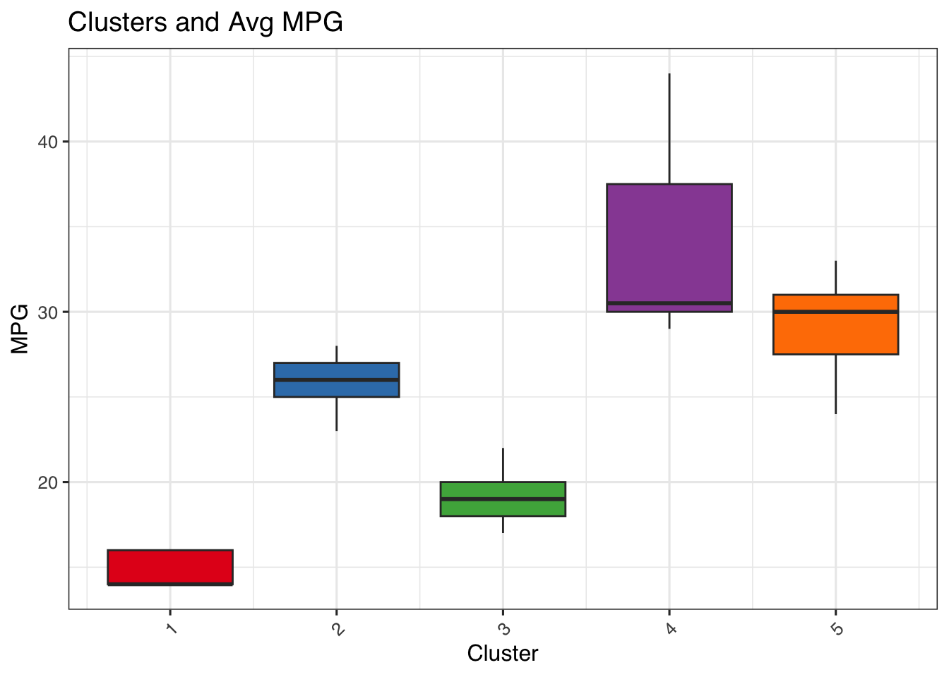
Just as a visual confirmation, let’s see what the ranges of the MPG is for these groups.
It’s quite clear that cluster 5 are the highest MPG vehicles, cluster 4 are the low MPG vehicles and include the Rolls Royce models. Kmeans is one of easiest clustering algorithm and there are many other unsupervised learning algorithms that will perform clustering. More on those in future posts.
ggplot(data, aes(x=k$cluster, y = comb08)) +
  geom_boxplot(aes(group = k$cluster, fill = as.factor(k$cluster)), show.legend = FALSE) +
  scale_fill_brewer(palette = "Set1") +
  labs(title = "Clusters and Avg MPG", x = "Cluster", y = "MPG")
Conclusion
In conclusion, we can say that the automotive world is undergoing a sea change and these are exciting times, it remains to be seen which fuel types dominate in the coming years; it’s clear that Gasoline as a fuel has had a great run and is by no means done.
