
Exploring crime in Philadelphia
This is a large and intersting dataset and has data points stretching back over 10 years. Several explorations have pointed out that crime seems to be seasonal and I wanted to explore this with a time series. Assuming that seasonal trends might repeat themselves, I am exploring this using the forecast package and using linear regression to predict trends.
suppressPackageStartupMessages({
  library(data.table)
  library(forecast)
  library(knitr)
})
Data size and structure.
mydt <- fread("~/data/crime.csv", showProgress = FALSE)
mydata <- as.data.frame(mydt)
dim(mydata)
## [1] 2174774 14
str(mydata)
## 'data.frame':	2174774 obs. of  14 variables:
##  $ Dc_Dist           : int  18 14 25 35 9 17 23 77 35 23 ...
##  $ Psa               : chr  "3" "1" "J" "D" ...
##  $ Dispatch_Date_Time: POSIXct, format: "2009-10-02 14:24:00" "2009-05-10 00:55:00" ...
##  $ Dispatch_Date     : IDate, format: "2009-10-02" "2009-05-10" ...
##  $ Dispatch_Time     : chr  "14:24:00" "00:55:00" "15:40:00" "01:09:00" ...
##  $ Hour              : int  14 0 15 1 0 12 14 18 1 20 ...
##  $ Dc_Key            :integer64 200918067518 200914033994 200925083199 200935061008 200909030511 201517017705 200923006310 200977001770 ...
##  $ Location_Block    : chr  "S 38TH ST  / MARKETUT ST" "8500 BLOCK MITCH" "6TH CAMBRIA" "5500 BLOCK N 5TH ST" ...
##  $ UCR_General       : int  800 2600 800 1500 2600 600 800 500 2600 2600 ...
##  $ Text_General_Code : chr  "Other Assaults" "All Other Offenses" "Other Assaults" "Weapon Violations" ...
##  $ Police_Districts  : int  NA NA NA 20 8 13 16 NA NA NA ...
##  $ Month             : chr  "2009-10" "2009-05" "2009-08" "2009-07" ...
##  $ Lon               : num  NA NA NA -75.1 -75.2 ...
##  $ Lat               : num  NA NA NA 40 40 ...
Extract the month as a new column
mydata$Dispatch_Date_Time <- as.POSIXct(mydata$Dispatch_Date_Time)
mydata$Month <- cut(mydata$Dispatch_Date_Time, breaks= "month")
Crimes by month
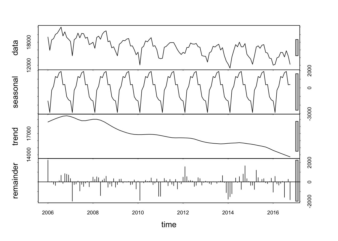
We can clearly see a downward trend in overall crime rates and also the fact that there seem to be seasonal peaks and declines.
bymo <- mydt[order(Month), .N, by=Month]
dts <- ts(bymo$N, start = c(2006,1), frequency = 12)
dts_decomp <- stl(dts, s.window = "period", robust = TRUE)
plot(dts,ylab="Total Crimes", main = "Monthly crimes with trend")
lines(dts_decomp$time.series[,2], col="tomato")

Seasonal component extracted from the timeseries.
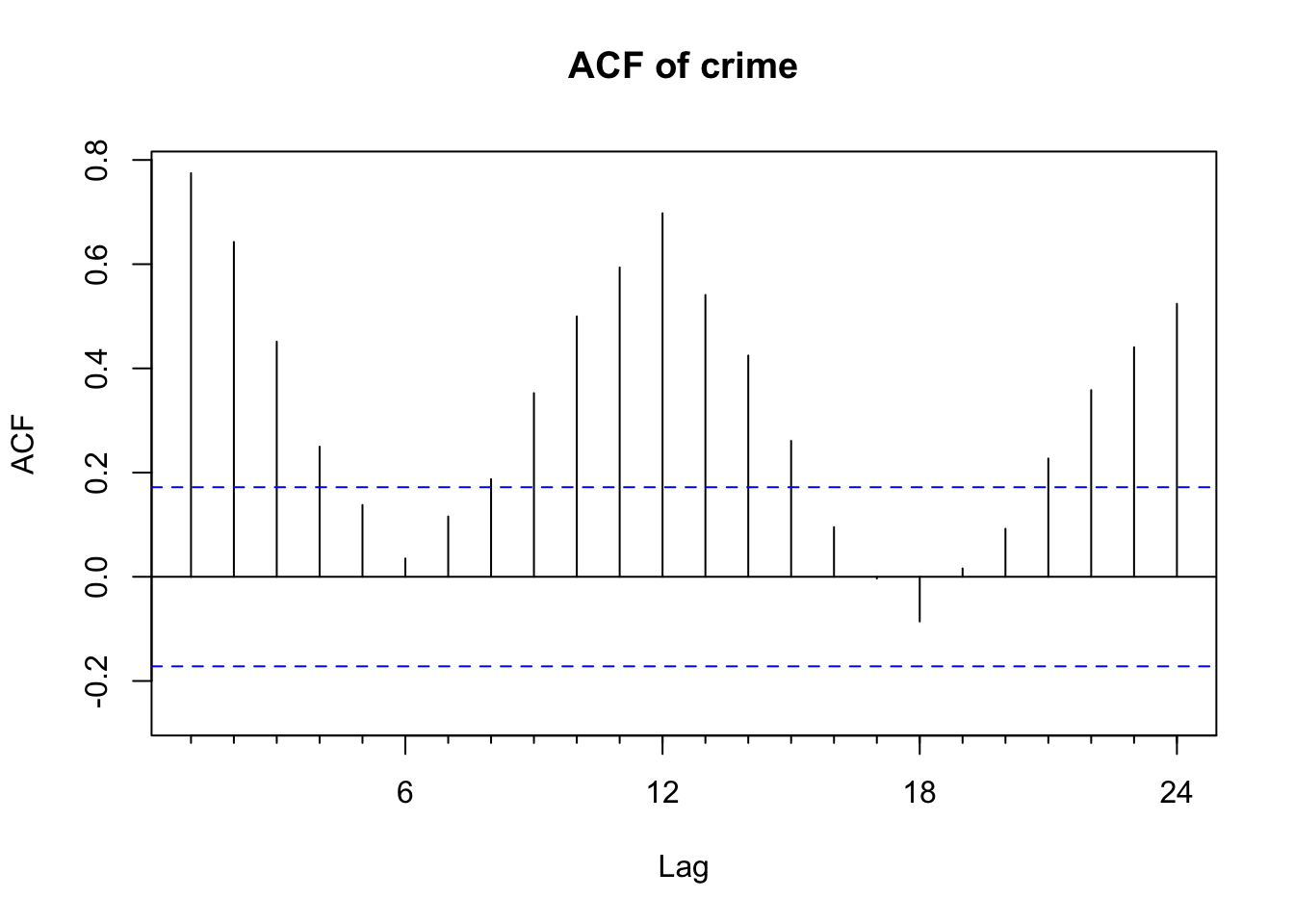
How seasonal is the data?
This autocorrelation shows a very high correalation every 12 months.
Acf(dts, main = "ACF of crime")
Forecast with a linear model
The red line shows the model’s prediction against the actual numbers in black. The model seems quite close.
f_crime <- tslm(dts ~ trend + season, lambda = 0.5)
ff_crime <- forecast(f_crime, h = 12)
plot(ff_crime)
lines(fitted(ff_crime), col = "red")

Residuals from model
This shows the residuals - these are quite low.
  res <- residuals(ff_crime)
  plot(res, ylab="Residuals",xlab="Year", main = "Residuals")

summary(res)
##     Min.  1st Qu.   Median     Mean  3rd Qu.     Max.
## -19.4127  -3.6751  -0.6624   0.0000   3.3571  17.2318
Predictions
If such a thing were possible - here are the predicted overall crime numbers.
ff_crime
##          Point Forecast    Lo 80    Hi 80    Lo 95    Hi 95
## Nov 2016       13236.78 12244.74 14267.46 11728.32 14836.48
## Dec 2016       12642.30 11673.23 13650.01 11169.13 14206.70
## Jan 2017       12455.98 11496.12 13454.31 10996.91 14005.90
## Feb 2017       11074.65 10170.69 12017.10  9701.46 12538.71
## Mar 2017       13602.72 12598.79 14645.12 12075.92 15220.37
## Apr 2017       14174.98 13149.75 15238.68 12615.45 15825.36
## May 2017       14987.78 13933.02 16081.02 13382.88 16683.54
## Jun 2017       14890.58 13839.31 15980.32 13291.04 16580.98
## Jul 2017       15276.38 14211.33 16379.91 13655.67 16987.95
## Aug 2017       15501.24 14428.24 16612.71 13868.30 17225.03
## Sep 2017       14087.42 13065.43 15147.90 12532.86 15732.85
## Oct 2017       14033.05 13013.06 15091.51 12481.58 15675.38
Next steps
- This took into account overall numbers but breaking down by category/Code and district might reveal other patterns.
