
Introduction
In this post I want to take a look at my Netflix viewing habits.
The first step is getting the data and you can request your viewing data from the Accounts section in your Netflix account. Netflix will allow you to download a zip file with many different ways to slice this information.
# Import the libraries
import pandas as pd
import numpy as np
import seaborn as sns
from pandas.api.types import CategoricalDtype
import matplotlib.pyplot as plt

from pathlib import Path

# Configure Visualization
plt.style.use('bmh')

# Configure Pandas and SKLearn
pd.set_option("display.max_colwidth", 20)
pd.set_option("display.precision", 3)


# File Specific Configurations
DATA_DIR = Path.home() / 'data/netflix-report'
plt.rcParams['figure.dpi'] = 300
START = pd.Timestamp.now()
SEED = 42
Explore the structure of the data
Let’s see what the downloaded data looks like - there are some folders and files.
# prefix components:
space =  '    '
branch = '│   '
# pointers:
tee =    '├── '
last =   '└── '


def tree(dir_path: Path, prefix: str=''):
    """A recursive generator, given a directory Path object
    will yield a visual tree structure line by line
    with each line prefixed by the same characters
    """
    contents = list(dir_path.iterdir())
    # contents each get pointers that are ├── with a final └── :
    pointers = [tee] * (len(contents) - 1) + [last]
    for pointer, path in zip(pointers, contents):
        yield prefix + pointer + path.name
        if path.is_dir(): # extend the prefix and recurse:
            extension = branch if pointer == tee else space
            # i.e. space because last, └── , above so no more |
            yield from tree(path, prefix=prefix+extension)

for line in tree(DATA_DIR):
    print(line)
## ├── MESSAGES
## │   └── MessagesSentByNetflix.csv
## ├── CONTENT_INTERACTION
## │   ├── MyList.csv
## │   ├── Ratings.csv
## │   ├── IndicatedPreferences.txt
## │   ├── PlaybackRelatedEvents.csv
## │   ├── ViewingActivity.csv
## │   ├── InteractiveTitles.csv
## │   └── SearchHistory.csv
## ├── .DS_Store
## ├── CUSTOMER_SERVICE
## │   ├── CSContact.txt
## │   └── ChatTranscripts.txt
## ├── IP_ADDRESSES
## │   ├── IpAddressesAccountCreation.txt
## │   ├── IpAddressesLogin.csv
## │   └── IpAddressesStreaming.csv
## ├── PAYMENT_AND_BILLING
## │   └── BillingHistory.csv
## ├── CLICKSTREAM
## │   └── Clickstream.csv
## ├── Additional Information.pdf
## ├── SURVEYS
## │   └── ProductCancellationSurvey.txt
## ├── PROFILES
## │   ├── Profiles.csv
## │   ├── AvatarHistory.csv
## │   └── ParentalControlsRestrictedTitles.txt
## ├── ACCOUNT
## │   ├── SubscriptionHistory.csv
## │   ├── ExtraMembers.txt
## │   ├── TermsOfUse.csv
## │   ├── AccountDetails.csv
## │   └── AccessAndDevices.csv
## ├── GAMES
## │   └── GamePlaySession.txt
## ├── Cover Sheet.pdf
## └── DEVICES
##     └── Devices.csv
The file we are interested in is ViewingActivity.csv
Read the data
df = pd.read_csv(DATA_DIR / "CONTENT_INTERACTION/ViewingActivity.csv", parse_dates=[1])
df = (
  df
  .assign(Duration = lambda x: pd.to_timedelta(x['Duration']),
          Bookmark = lambda x: pd.to_timedelta(x['Bookmark']),
          StartTime = df['Start Time'].dt.tz_localize(tz='UTC', nonexistent=pd.Timedelta('1H')).dt.tz_convert('US/Pacific') )
)
def inspect_columns(df):
    # A helper function that does a better job than df.info() and df.describe()
    result = pd.DataFrame({
        'unique': df.nunique() == len(df),
        'cardinality': df.nunique(),
        'with_null': df.isna().any(),
        'null_pct': round((df.isnull().sum() / len(df)) * 100, 2),
        '1st_row': df.iloc[0],
        'last_row': df.iloc[-1],
        'dtype': df.dtypes
    })
    return result
Let’s inspect the data
df.head
## <bound method NDFrame.head of       Profile Name          Start Time  ...             Country            StartTime
## 0            Guest 2023-08-26 00:23:06  ...  US (United States) 2023-08-25 17:23:...
## 1            Guest 2023-08-26 00:22:00  ...  US (United States) 2023-08-25 17:22:...
## 2            Guest 2023-08-25 23:59:09  ...  US (United States) 2023-08-25 16:59:...
## 3            Guest 2022-09-14 23:28:59  ...  US (United States) 2022-09-14 16:28:...
## 4            Guest 2022-09-14 22:03:41  ...  US (United States) 2022-09-14 15:03:...
## ...            ...                 ...  ...                 ...                  ...
## 26530          avi 2017-07-29 06:36:06  ...          IN (India) 2017-07-28 23:36:...
## 26531          avi 2017-07-29 06:22:57  ...          IN (India) 2017-07-28 23:22:...
## 26532          avi 2017-07-29 02:46:29  ...          IN (India) 2017-07-28 19:46:...
## 26533          avi 2017-07-29 02:45:55  ...          IN (India) 2017-07-28 19:45:...
## 26534          avi 2017-07-28 18:06:08  ...          IN (India) 2017-07-28 11:06:...
##
## [26535 rows x 11 columns]>
inspect_columns(df)
##                       unique  ...                dtype
## Profile Name           False  ...               object
## Start Time             False  ...       datetime64[ns]
## Duration               False  ...      timedelta64[ns]
## Attributes             False  ...               object
## Title                  False  ...               object
## Supplemental Vide...   False  ...               object
## Device Type            False  ...               object
## Bookmark               False  ...      timedelta64[ns]
## Latest Bookmark        False  ...               object
## Country                False  ...               object
## StartTime              False  ...  datetime64[ns, U...
##
## [11 rows x 7 columns]
# The column list
df.dtypes
## Profile Name                            object
## Start Time                      datetime64[ns]
## Duration                       timedelta64[ns]
## Attributes                              object
## Title                                   object
## Supplemental Video Type                 object
## Device Type                             object
## Bookmark                       timedelta64[ns]
## Latest Bookmark                         object
## Country                                 object
## StartTime                  datetime64[ns, U...
## dtype: object
Data Cleaning
The Title and Supplemental Video Type are useful data - but it does not have a video type associated with actual content, only Hooks, trailers etc are marked as such.
We will fill in the NaN values with the word CONTENT and convert this to a categorical type to make it easier to analyze.
cats = [ 'Monday', 'Tuesday', 'Wednesday', 'Thursday', 'Friday', 'Saturday', 'Sunday']
cat_type = CategoricalDtype(categories=cats, ordered=True)

df['Supplemental Video Type'].value_counts(dropna = False)
## Supplemental Video Type
## NaN               23807
## HOOK               1988
## TRAILER             592
## TEASER_TRAILER      115
## RECAP                17
## PREVIEW               7
## PROMOTIONAL           6
## BIG_ROW               2
## BUMPER                1
## Name: count, dtype: int64
content_cats = ['Movie', 'Series']
content_cat_type = CategoricalDtype(categories=content_cats)

df = (df
  .assign(type = df['Supplemental Video Type']
  .fillna('CONTENT')
  .astype('category'))
  .assign(dow = df['StartTime'].dt.strftime('%A').astype(cat_type),
  hour = df['StartTime'].dt.hour,
  year = df['StartTime'].dt.year,
  month = df['StartTime'].dt.month,
  duration_sec = df['Duration'].dt.total_seconds(),
  duration_min_bin = pd.cut(df['Duration'].dt.total_seconds()//60, bins=[0,20,40,60,80,100,120,140,np.inf], labels=['0-20', '20-40', '40-60', '60-80', '80-100', '100-2h', '2h-2:20', '2:20+'], include_lowest=True),
  c_type = np.where(df['Title'].str.contains('episode', case=False, regex=False), "Series", "Movie"))
)
df['type'].value_counts(dropna = False)
## type
## CONTENT           23807
## HOOK               1988
## TRAILER             592
## TEASER_TRAILER      115
## RECAP                17
## PREVIEW               7
## PROMOTIONAL           6
## BIG_ROW               2
## BUMPER                1
## Name: count, dtype: int64
We can see that we have watched 23807 real pieces of content. These include shows or movies that have been viewed multiple times or over more than 1 viewing session.
TV Watching habits
Shows and Movies
The first thing we want to see is how many unique pieces of content have we watched.
content_df = (df
.query('type == "CONTENT"')
)

#Number of unique content
(df
.filter(['Title'])
.nunique()
)
## Title    12890
## dtype: int64
# Total Number of hours watched
(df
.filter(['Duration'])
.sum()
)
## Duration   361 days 04:38:22
## dtype: timedelta64[ns]
# Length of membership
days = (df['Start Time'].max() - content_df['Start Time'].min()).days
years = days//365
months = (days % 365)//30

print(f"Length of Membership - {years} Years {months} Months")
## Length of Membership - 14 Years 9 Months
Let’s put some of this on a plot to see when we consume most content. This is over a 14 year period.
# Add day of week to data and extract hour from start time.

time_df = (content_df
  .groupby(content_df['StartTime'].dt.year
  )['Duration']
  .sum()

).reset_index().assign(hours = lambda x: x['Duration'].dt.total_seconds()//3600)

time_df.plot(kind="bar", x = "StartTime", y = "hours", xlabel="Year", title="Total time watched")
plt.show()
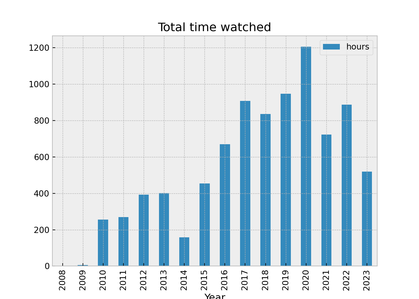
Looking at the plot above - it’s clear that TV watching peaked during the pandemic and we averaged about 3 hours a day, but it had been trending upward steadily. We seem to be coming back down slowly.
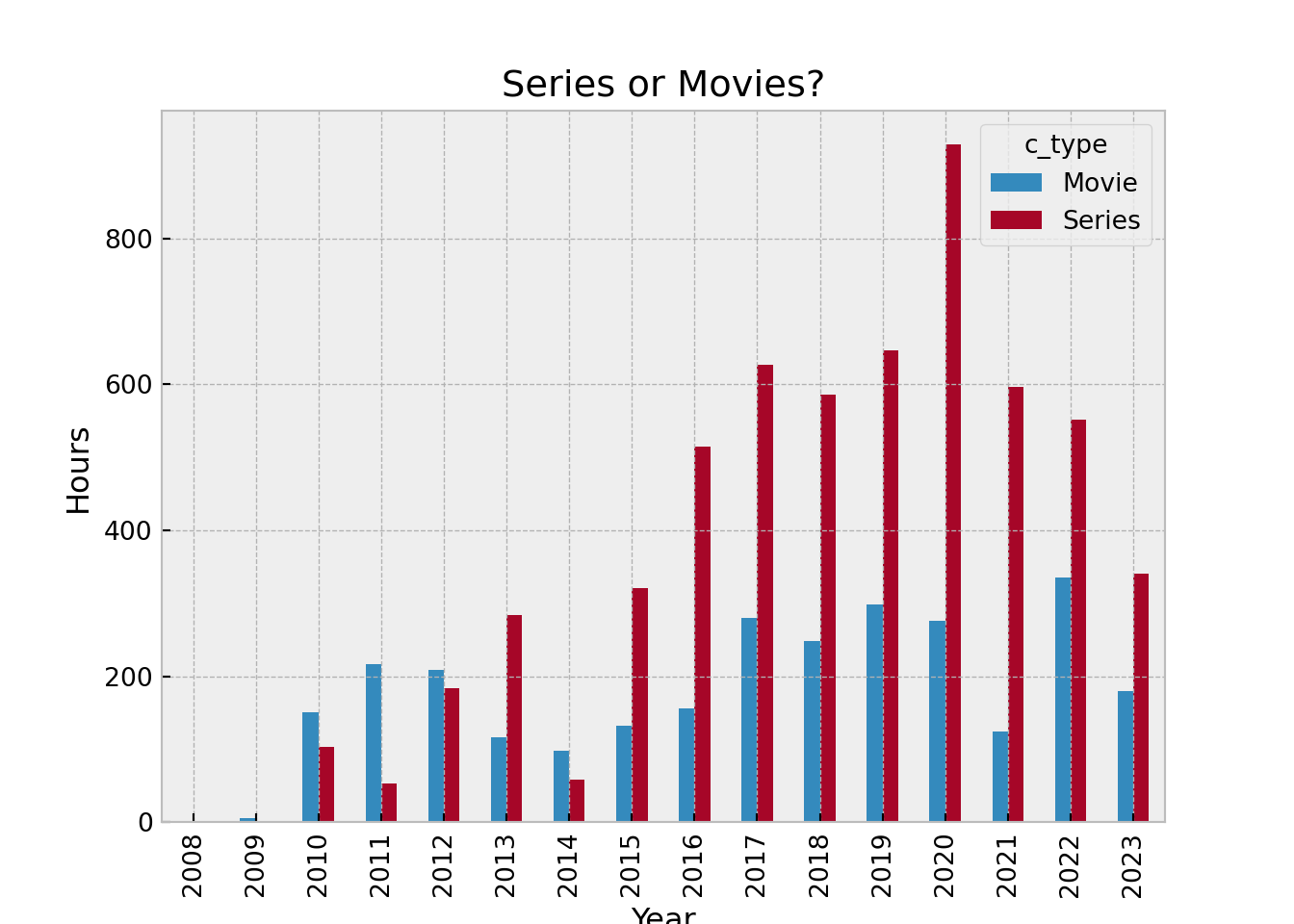
Shows or Movies
Next we want to see how many different pieces of content did we view, we want to see episodic shows vs movies. It’s a shame that Netflix does not include any additional metadata around this data dump. We’ll have to extract some information by cleaning this data set. Luckily, all series include the word “Episode” - so we are able to use that to understand that we have watched almost three times series than movies.
(content_df
  .assign(hours = df['Duration'].dt.total_seconds())
  .groupby([content_df['StartTime'].dt.year, 'c_type'])['hours']
  .sum()//3600).unstack().reset_index().plot.bar( x = "StartTime", stacked=False, xlabel="Year", ylabel="Hours", title="Series or Movies?")

plt.show()
TV viewing times
I want to see what days and times are peak TV watching times. This can be visualized with a heatmap. We have extracted the days and hours already in the dataframe.
import warnings
with warnings.catch_warnings():
    warnings.simplefilter(action='ignore', category=FutureWarning)
    # Warning-causing lines of code here
    hmap_df = (
      content_df
      .assign(hours = lambda x: x['Duration'].dt.total_seconds())
      .groupby(['hour', 'dow'])['hours']
      .sum()//3600).unstack()
    sns.heatmap(data=hmap_df, cmap = 'viridis')
    plt.legend('',frameon=False)
    plt.show()
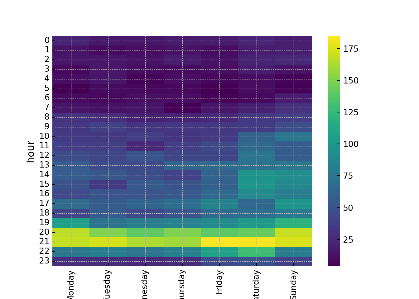
It’s clear that the weekends and the evening hours were peak TV watching periods.
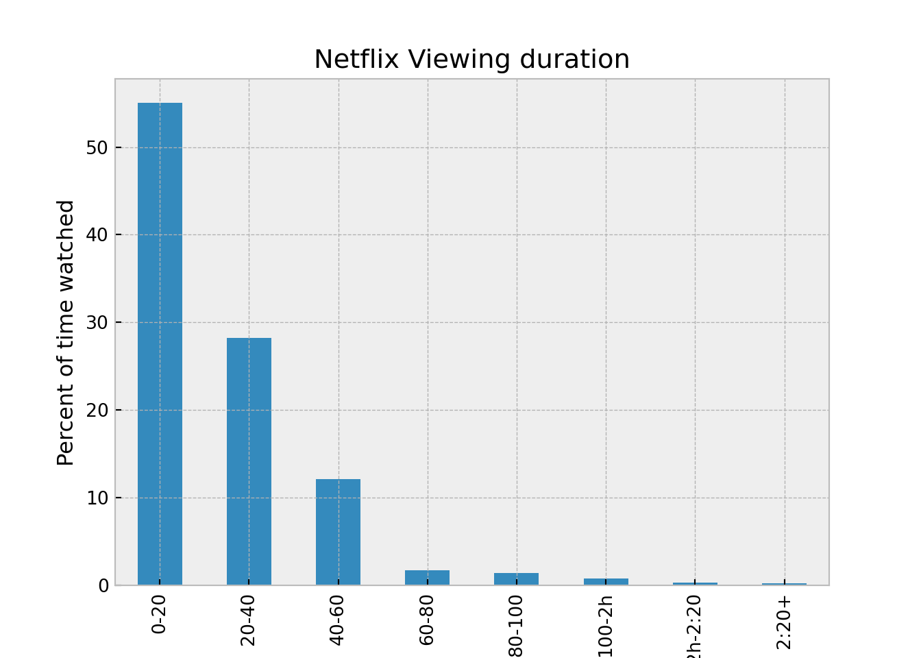
Netflix viewing duration
I know we don’t watch TV for too long at a stretch - the duration field shows how much of a show we watched. This gives us an estimate of how many minutes or hours we watch at a single sitting. We’ll use cuts to create blocks of time - 20 minutes per block. It looks like we watch TV in short blocks or content that’s about 20 minutes long - over 50% of the time.
with warnings.catch_warnings():
    warnings.simplefilter(action='ignore', category=FutureWarning)
    (content_df
    .groupby('duration_min_bin')['c_type']
    .count()/content_df.c_type.count()*100).reset_index().plot.bar(x='duration_min_bin', ylabel="Percent of time watched", xlabel="Minutes watched", title="Netflix Viewing duration")

    plt.legend('',frameon=False)
    plt.show()
Conclusion
This was a very quick exploration into the my Netflix viewing data. I wish they had added genres and synopsis, we would have been able to extract more details about my viewing habits. Will try to merge data from a film archive to do addtional analysis next time.
