
Revenue forecasting with linear methods.
This post highlights linear regression techniques on time series data. We have some weekly sales data from a small business that is expected to have seasonal trends. A bike rental business in a major tourist city. Let’s dive into the data. Load up the required packages.
suppressPackageStartupMessages({
  library(forecast)
})
Load the data, we have two columns with weekly revenue numbers from two different sources. Online and Phone; these correspond to sales online and via phone call to the business.
  filename <- '~/data/BikeTours.csv'

    # Read up the data file - first line is the header
    d <- read.csv(filename, header = TRUE)

    # Get the seller name
    sellerName <- gsub("/|~.*data|.csv", "", filename)
    str(d)
## 'data.frame':	220 obs. of  2 variables:
##  $ Online: num  0.001 0.001 104 442 156 52 312 0.001 0.001 854 ...
##  $ Phone : num  0.001 0.001 0.001 0.001 44.5 0.001 0.001 141 0.001 0.001 ...
The weekly revenue for BikeTours
Timeseries
Let start by creating a timeseries object using the ts() function and has the signature ts(vector, start=,end=,frequency) where start and end are times of the first and last observation and frequency is the number of observations per unit time (1=annual, 4=quarterly, 12=monthly).
In our case we have weekly data, therefore we will set our frequncy to 52.
  d_ts <- ts(d, start = c(2012,1), frequency = 52)
summary(d_ts)
##      Online             Phone
##  Min.   :   0.001   Min.   :   0.001
##  1st Qu.: 211.000   1st Qu.:   0.001
##  Median :1824.500   Median : 191.500
##  Mean   :1959.751   Mean   : 333.967
##  3rd Qu.:3112.500   3rd Qu.: 571.875
##  Max.   :8505.000   Max.   :1733.000
Online and Phone revenue
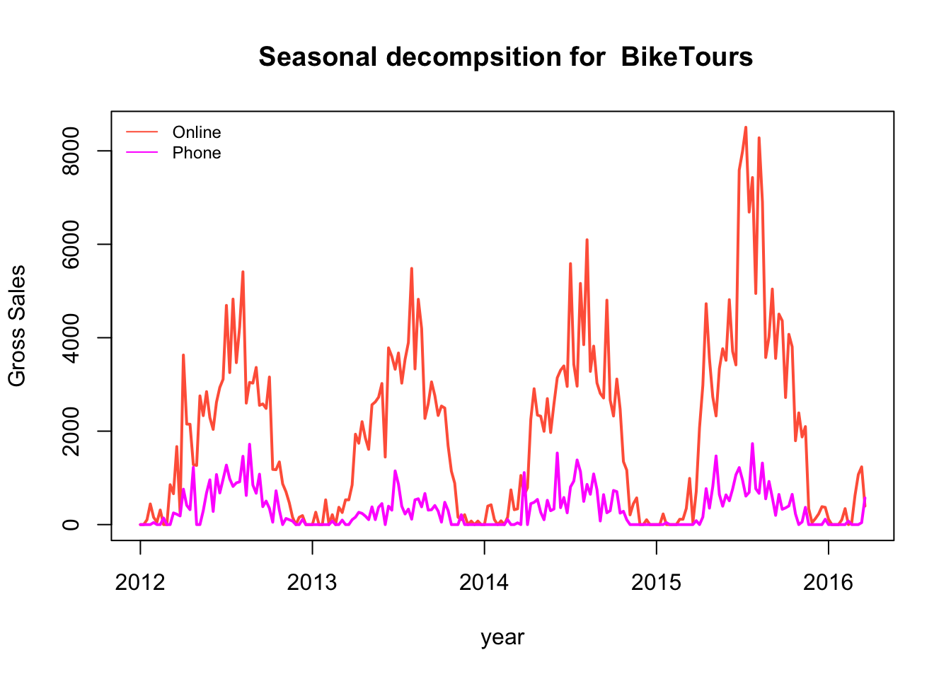
Let’s look at the weekly sales split out by mode of purchase Online vs Phone. Online sales are the primary component of sales. For the next few sections we will focus on the Online component. The same analysis and forecast can be done for the Phone component.
  title <- paste(" Seasonal decompsition for ", sellerName)
  ts.plot(d_ts, gpars = list(col=c("tomato", "magenta"), lwd=2, ylab="Gross Sales", xlab="year", main = title))
    legend('topleft' ,legend=c("Online", "Phone"), lty=1, col=c("tomato", "magenta"), bty='n', cex=.75)
Online Revenue
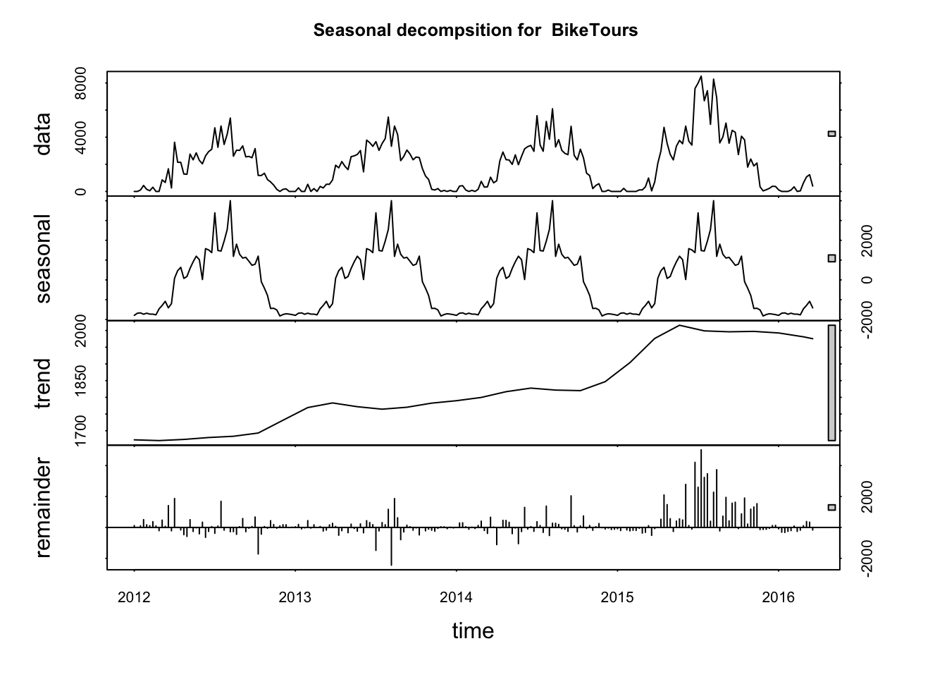
Seasonal component extraction.
When a time series varies according to a periodic component, we can extract the periodicty using classical statistical methods. The stl() function in core R uses loess to effectively take the means of each period. The seasonal component is removed and the remainder is smoothed to find the trend. The sales are clearly seasonal with peaks in the middle of the year starting near spring break and ending near thanksgiving.
Weekly revenue with the seasonal component extracted
  d_online <- d$Online
  d_ts_online <- ts(d_online, start = c(2012,1), frequency = params$freq)
  d_ts_comp_online <- stl(d_ts_online, s.window = "period", robust = TRUE)

  plot(d_ts_comp_online, main = title)
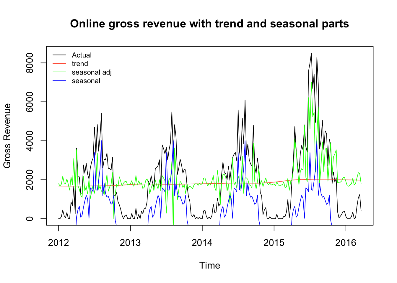
Let’s combine this into a single plot. We have also extracted the seasonally adjusted numbers to show the actual variations and trends.
  plot(d_ts_online, ylab="Gross Revenue", main = "Online gross revenue with trend and seasonal parts")
  lines(d_ts_comp_online$time.series[,2], col="tomato")
  lines(seasadj(d_ts_comp_online), col="green")
  lines(d_ts_comp_online$time.series[,1], col="blue")
  legend('topleft' ,legend=c("Actual", "trend", "seasonal adj", "seasonal"), lty=1, col=c("black", "tomato", "green", "blue"), bty='n', cex=.75)
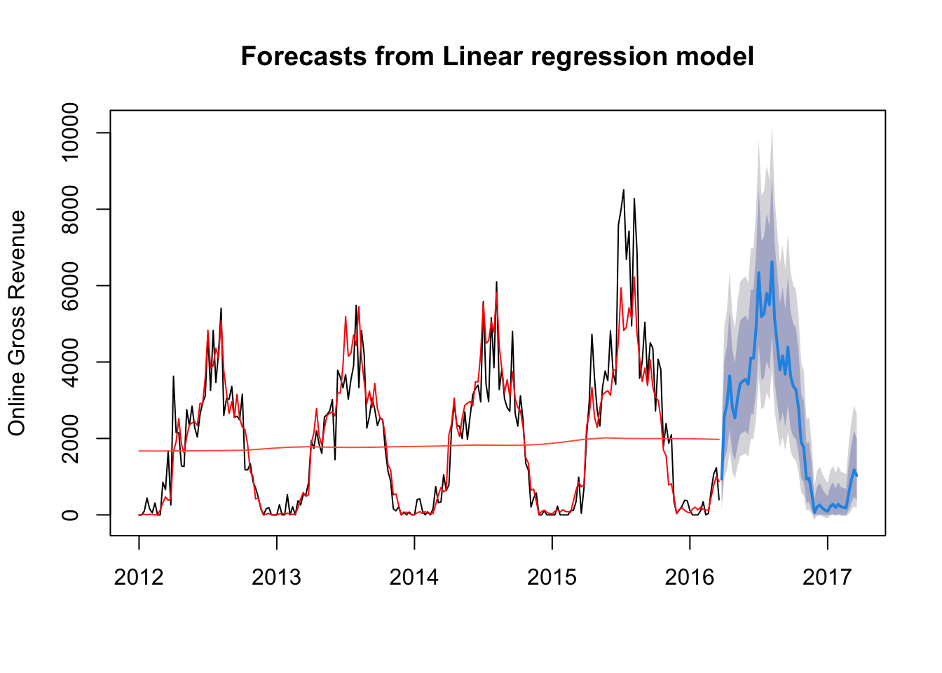
Forecast using linear regression
This is the forecast for revenue taking seasonality into account. The function tslm() is the linear regression version for time series data.
Note the red line shows the model’s predicted numbers.
    f_online<-tslm(d_ts_online ~ trend + season, lambda = 0.5)
    ff_online <- forecast(f_online, h=params$freq)
    plot(ff_online,  ylab="Online Gross Revenue")
    lines(fitted(ff_online), col="red")
    lines(d_ts_comp_online$time.series[,2], col="tomato")
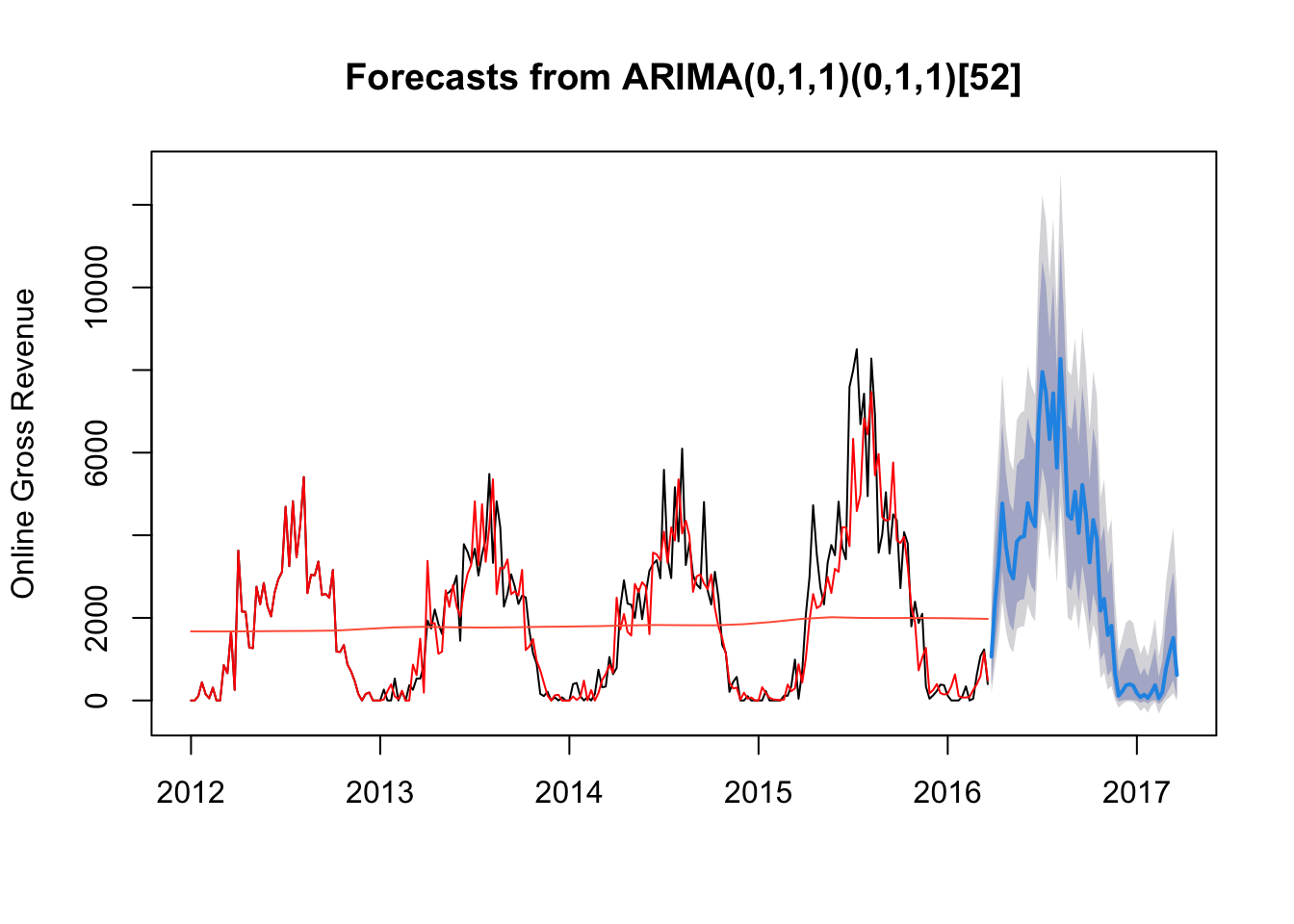
Forecast using ARIMA models
Let’s also use the [ARIMA](https://en.wikipedia.org/wiki/Autoregressive_integrated_moving_average Wikipedia) model to get a forecast. Note that the D=1 parameter forces the model to take seasonality into account.
    f_online_arima <-auto.arima(d_ts_online, lambda = 0.5, D=1)
    ff_online_arima <- forecast(f_online_arima, h=params$freq)
    plot(ff_online_arima,  ylab="Online Gross Revenue")
    lines(fitted(ff_online_arima), col="red")
    lines(d_ts_comp_online$time.series[,2], col="tomato")
Residuals
The residuals - the difference between the actual and predicted values back fitted. Low numbers are indicative of a good fit. A 0 mean is indicative of an unbiased forecast.
  res <- residuals(ff_online)
  plot(res, ylab="Residuals",xlab="Year", main = paste("Residuals for ", sellerName) )
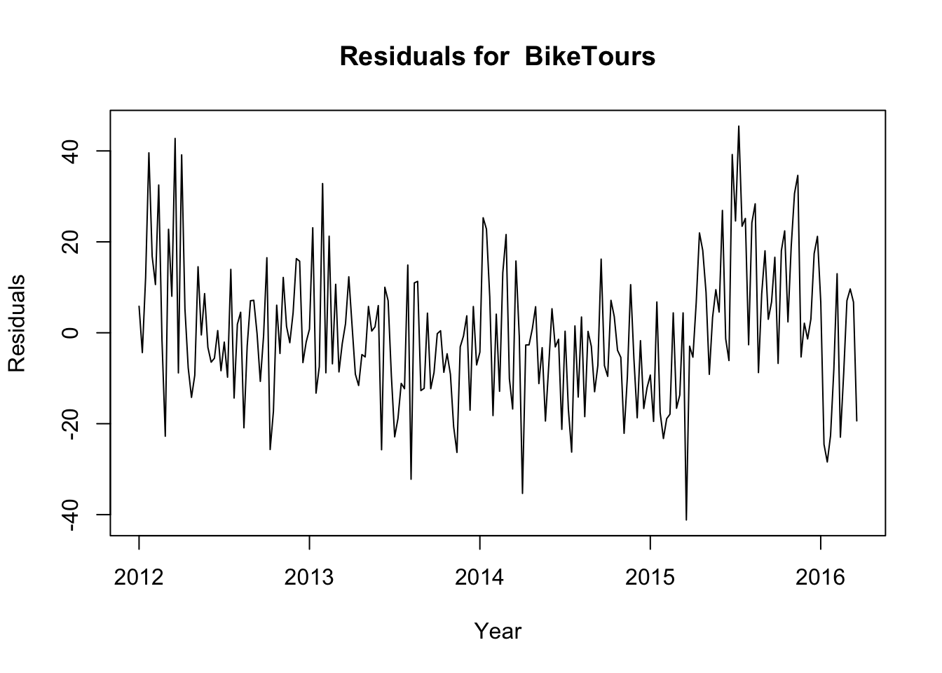
summary(res)
##    Min. 1st Qu.  Median    Mean 3rd Qu.    Max.
## -41.166  -9.406  -1.330   0.000   8.180  45.450
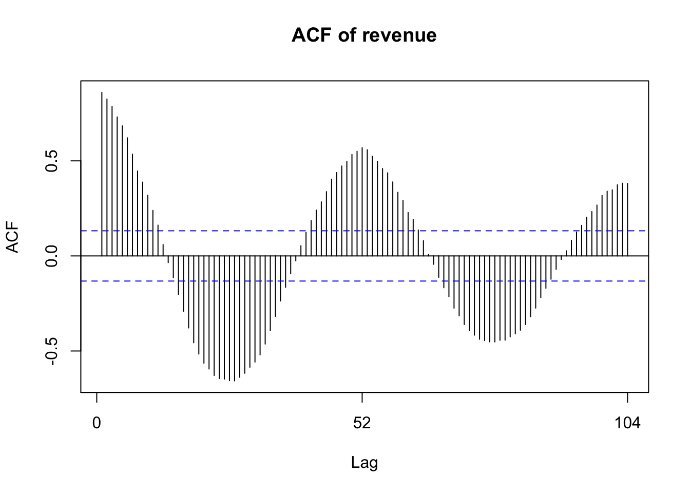
Autocorrelation
The autocorrelation shows the correlation between seasonal data, peaks show positive correlation at the marked intervals. ( 52 weeks, so yearly correlation is statistically signficant - i.e. above the blue line)
Acf(d_ts_online , main="ACF of revenue")
This is the weekly revenue prediction using this model
ff_online
##          Point Forecast        Lo 80     Hi 80       Lo 95      Hi 95
## 2016.231      932.32319  318.4182798 1868.2845  122.377409  2500.5504
## 2016.250     2578.50032 1450.7906998 4028.2664  980.153309  4935.1287
## 2016.269     2899.35343 1693.8126535 4426.9506 1181.579368  5375.4089
## 2016.288     3636.01505 2266.6825172 5327.4040 1666.912767  6363.3987
## 2016.308     2811.32749 1626.6914914 4318.0199 1125.630506  5255.3059
## 2016.327     2534.91901 1418.1468035 3973.7476  953.354775  4874.7646
## 2016.346     3060.37223 1817.3972106 4625.4037 1285.157659  5593.8682
## 2016.365     3436.28453 2109.5778794 5085.0476 1532.589002  6098.2615
## 2016.385     3496.85664 2157.0949601 5158.6747 1573.128986  6178.8657
## 2016.404     3544.38422 2194.4579606 5216.3669 1605.059651  6241.9902
## 2016.423     3417.33077 2094.7327927 5061.9852 1519.939747  6073.0032
## 2016.442     4106.06462 2640.8182622 5893.3674 1989.788563  6980.6221
## 2016.462     4100.72397 2636.5355784 5886.9688 1986.071299  6973.6580
## 2016.481     4906.16729 3289.5213509 6844.8697 2557.578032  8013.0379
## 2016.500     6338.84958 4479.2505450 8520.5050 3617.463974  9818.5166
## 2016.519     5186.98677 3520.1734058 7175.8566 2761.418733  8370.8362
## 2016.538     5270.49922 3589.0301382 7274.0247 2822.442901  8476.8369
## 2016.558     5797.34323 4025.9782912 7890.7646 3211.347336  9141.6205
## 2016.577     5501.54321 3780.1223019 7545.0205 2992.183310  8769.1845
## 2016.596     6625.44928 4720.6757023 8852.2793 3834.746161 10174.4338
## 2016.615     5116.51520 3462.1610316 7092.9258 2710.065021  8281.2468
## 2016.635     4448.71331 2916.9705965 6302.5125 2230.402750  7425.3053
## 2016.654     3794.23255 2391.9585078 5518.5630 1774.583579  6572.1629
## 2016.673     4162.58023 2686.1801445 5961.0367 2029.189479  7054.2524
## 2016.692     3681.91917 2302.9566493 5382.9381 1698.040275  6424.0795
## 2016.712     4390.17215 2869.6040100 6232.7967 2189.008275  7349.6174
## 2016.731     3632.94408 2264.2579505 5323.6866 1664.833664  6359.3359
## 2016.750     3369.14148 2057.0412819 5003.2981 1487.858639  6008.7057
## 2016.769     3282.84745 1989.7352906 4898.0160 1430.700569  5893.2757
## 2016.788     2810.32651 1625.9300943 4316.7793 1124.997152  5253.9373
## 2016.808     1909.04629  961.1825996 3178.9664  586.661624  3989.7123
## 2016.827     1755.20285  852.9584196 2979.5037  502.818088  3765.8690
## 2016.846      931.63616  318.0168235 1867.3119  122.128578  2499.4251
## 2016.865      962.29862  336.0346946 1910.6190  133.388706  2549.4899
## 2016.885      560.41274  120.6339549 1322.2479   17.652625  1861.4542
## 2016.904       63.23344  -22.4462142  426.0771 -132.700951   752.0473
## 2016.923      208.05583    3.0083216  735.1598  -25.476195  1148.9169
## 2016.942      259.64447   11.7223916  829.6230  -11.276489  1266.2938
## 2016.962      179.62121    0.5077909  680.7911  -36.835817  1080.6880
## 2016.981      123.96826   -2.4198465  567.5731  -69.512770   936.7052
## 2017.000       94.68002   -7.5661760  493.3463  -88.755270   834.1545
## 2017.019      219.76105    5.4910801  745.5834  -18.723170  1154.3487
## 2017.038      280.90078   18.3103595  855.0436   -5.718185  1289.6331
## 2017.058      191.89206    1.8809485  693.4556  -28.077880  1089.2560
## 2017.077      279.04190   17.8380613  851.7982   -5.986930  1285.6466
## 2017.096      210.92247    4.1703189  729.2271  -21.420211  1133.9745
## 2017.115      196.93559    2.4097589  703.0138  -26.193857  1101.2271
## 2017.135      183.21704    1.1124655  676.8741  -31.534946  1068.4489
## 2017.154      577.11718  133.2230499 1332.5637   23.735368  1864.0487
## 2017.173      927.77902  323.2239800 1843.8865  127.873075  2461.2347
## 2017.192     1177.07497  476.4394082 2189.2630  229.739463  2857.9602
## 2017.212     1031.06060  385.3014920 1988.3721  167.929587  2627.7414
